PHQ-4-R - Data Cleaning (Study 2)

Data Preparation

Code

library(tidyverse)
library(easystats)
library(patchwork)
library(ggside)

df <- read.csv("../data/data_raw.csv") |> 
  mutate(across(everything(), ~ifelse(.x == "", NA, .x))) |> 
  filter(Age >= 18) |> 
  mutate(Age = ifelse(Age > 90, NA, Age))

The initial sample consisted of 1053 participants (Mean age = 24.1, SD = 10.5, range: [18, 76], 9.5e-02% missing; Gender: 75.6% women, 21.0% men, 2.56% non-binary, 0.85% missing; Education: Bachelor, 22.41%; Doctorate, 1.90%; High School, 65.53%; Master, 5.22%; missing, 0.28%; Other, 4.65%).

Recruitment History

Code

# Consecutive count of participants per day (as area)
df |>
  mutate(Date = as.Date(Date, format = "%d/%m/%Y")) |> 
  group_by(Date, Experimenter) |> 
  summarize(N = n()) |> 
  ungroup() |>
  complete(Date, Experimenter, fill = list(N = 0)) |> 
  group_by(Experimenter) |>
  mutate(N = cumsum(N)) |>
  ggplot(aes(x = Date, y = N)) +
  geom_area(aes(fill=Experimenter)) +
  scale_y_continuous(expand = c(0, 0)) +
  labs(
    title = "Recruitment History",
    x = "Date",
    y = "Total Number of Participants"
  ) +
  see::theme_modern()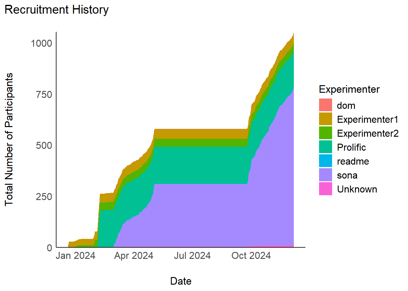

Code

# Table
summarize(df, N = n(), .by=c("Experimenter")) |> 
  arrange(desc(N)) |> 
  gt::gt() |> 
  gt::opt_stylize() |> 
  gt::opt_interactive(use_compact_mode = TRUE) |> 
  gt::tab_header("Number of participants per recruitment source")

Number of participants per recruitment source

df$Sample <- case_when(
  df$Experimenter %in% c("Experimenter1", "Experimenter2") ~ "Student",
  df$Experimenter %in% c("dom", "Unknown", "readme") ~ "Other",
  .default = df$Experimenter
)

Experiment Duration

The experiment’s median duration is 9.95 min (50% HDI [5.61, 11.80]).

Code

df |>
  mutate(Participant = fct_reorder(Participant, Experiment_Duration),
         Category = ifelse(Experiment_Duration > 30, "extra", "ok"),
         Duration = ifelse(Experiment_Duration > 30, 30, Experiment_Duration)) |>
  ggplot(aes(y = Participant, x = Duration)) +
  geom_vline(xintercept = median(df$Experiment_Duration), color = "red", linetype = "dashed") +
  geom_point(aes(color = Sample, shape = Category)) +
  geom_text(aes(color = Sample, label=ifelse(Experiment_Duration < 3, as.character(Participant), '')), hjust=-1, vjust=0) +
  scale_shape_manual(values = c("extra" = 3, ok = 19)) +
  guides(shape = "none") +
  ggside::geom_xsidedensity(aes(fill=Sample), color=NA, alpha=0.5) +
  ggside::scale_xsidey_continuous(expand = c(0, 0)) +
  labs(
    title = "Experiment Completion Time",
    x = "Duration (in minutes)",
    y = "Participant"
  )  +
  theme_bw() +
  ggside::theme_ggside_void() +
  theme(ggside.panel.scale = .3,
        panel.border = element_blank(),
        axis.ticks.y = element_blank(),
        axis.text.y = element_blank())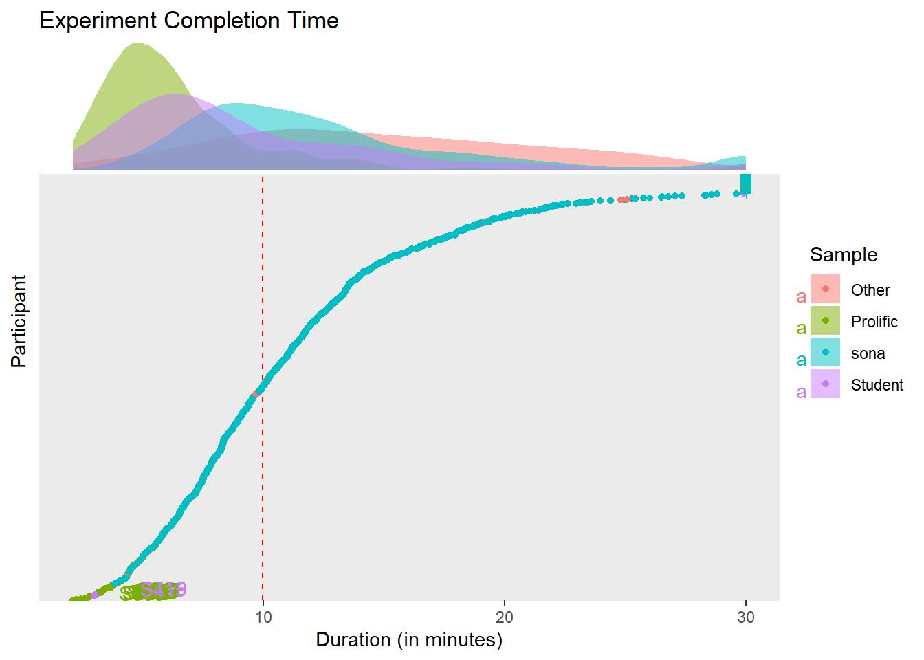

Compute Scores

PHQ-4

Code

recode_phq <- function(x) {
  case_when(
    x == 1 ~ 0.5,
    x == 2 ~ 1,
    x == 3 ~ 2,
    x == 4 ~ 3,
    .default = x
  )
}

df <- df |>
  mutate(
    PHQ4_Anxiety_1 = ifelse(PHQ4_Condition == "PHQ4 - Revised", recode_phq(PHQ4_Anxiety_1), PHQ4_Anxiety_1),
    PHQ4_Anxiety_2 = ifelse(PHQ4_Condition == "PHQ4 - Revised", recode_phq(PHQ4_Anxiety_2), PHQ4_Anxiety_2),
    PHQ4_Depression_3 = ifelse(PHQ4_Condition == "PHQ4 - Revised", recode_phq(PHQ4_Depression_3), PHQ4_Depression_3),
    PHQ4_Depression_4 = ifelse(PHQ4_Condition == "PHQ4 - Revised", recode_phq(PHQ4_Depression_4), PHQ4_Depression_4),
    PHQ4_Anxiety = PHQ4_Anxiety_1 + PHQ4_Anxiety_2,
    PHQ4_Depression = PHQ4_Depression_3 + PHQ4_Depression_4,
    PHQ4_Total = PHQ4_Anxiety + PHQ4_Depression
  )


df <- df |>
  mutate(
    Weighted_PHQ4_Anxiety_1 = ifelse(
      PHQ4_Condition == "PHQ4 - Revised",
      case_when(
        PHQ4_Anxiety_1 == 0 ~ 0,
        PHQ4_Anxiety_1 == 0.5 ~ 0.34,
        PHQ4_Anxiety_1 == 1 ~ 0.55,
        PHQ4_Anxiety_1 == 2 ~ 0.71,
        PHQ4_Anxiety_1 == 3 ~ 1,
        .default = PHQ4_Anxiety_1
      ), PHQ4_Anxiety_1
    ),
    Weighted_PHQ4_Anxiety_2 = ifelse(
      PHQ4_Condition == "PHQ4 - Revised",
      case_when(
        PHQ4_Anxiety_2 == 0 ~ 0,
        PHQ4_Anxiety_2 == 0.5 ~ 0.44,
        PHQ4_Anxiety_2 == 1 ~ 0.58,
        PHQ4_Anxiety_2 == 2 ~ 0.71,
        PHQ4_Anxiety_2 == 3 ~ 1,
        .default = PHQ4_Anxiety_2
      ), PHQ4_Anxiety_2
    ),
    Weighted_PHQ4_Depression_3 = ifelse(
      PHQ4_Condition == "PHQ4 - Revised",
      case_when(
        PHQ4_Depression_3 == 0 ~ 0,
        PHQ4_Depression_3 == 0.5 ~ 0.38,
        PHQ4_Depression_3 == 1 ~ 0.51,
        PHQ4_Depression_3 == 2 ~ 0.62,
        PHQ4_Depression_3 == 3 ~ 1,
        .default = PHQ4_Depression_3
      ), PHQ4_Depression_3
    ),
    Weighted_PHQ4_Depression_4 = ifelse(
      PHQ4_Condition == "PHQ4 - Revised",
      case_when(
        PHQ4_Depression_4 == 0 ~ 0,
        PHQ4_Depression_4 == 0.5 ~ 0.35,
        PHQ4_Depression_4 == 1 ~ 0.52,
        PHQ4_Depression_4 == 2 ~ 0.66,
        PHQ4_Depression_4 == 3 ~ 1,
        .default = PHQ4_Depression_4
      ), PHQ4_Depression_4
    ),
    Weighted_PHQ4_Anxiety = ifelse(
      PHQ4_Condition == "PHQ4 - Revised", datawizard::rescale(Weighted_PHQ4_Anxiety_1 + Weighted_PHQ4_Anxiety_2, range = c(0, 2), to = c(0, 6)), PHQ4_Anxiety_1 + PHQ4_Anxiety_2
    ),
    Weighted_PHQ4_Depression = ifelse(
      PHQ4_Condition == "PHQ4 - Revised", datawizard::rescale(Weighted_PHQ4_Depression_3 + Weighted_PHQ4_Depression_4, range = c(0, 2), to = c(0, 6)), PHQ4_Depression_3 + PHQ4_Depression_4
    ),
    Weighted_PHQ4_Total = Weighted_PHQ4_Anxiety + Weighted_PHQ4_Depression
  )

# df |>
#   select(starts_with("Weighted_PHQ4_"), PHQ4_Condition) |>
#   pivot_longer(cols = -PHQ4_Condition, names_to = "item", values_to = "score") |>
#   ggplot(aes(x = score)) +
#   geom_density(fill="#9C27B0", adjust=1/2)  +
#   facet_grid(item ~ PHQ4_Condition)

Code

df |>
  select(starts_with("PHQ4_")) |>
  pivot_longer(cols = matches("Depression_|Anxiety_"), names_to = "item", values_to = "score") |>
  ggplot(aes(x = as.factor(score))) +
  geom_bar(stat="count", fill="#9C27B0") +
  facet_grid(item ~ PHQ4_Condition) +
  labs(x = "Score", y = "N answers") +
  theme_bw()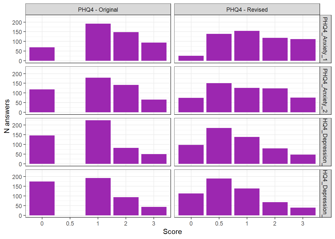

STAI-5

Code

df |>
  select(matches("STAI5_"), -STAI5_Duration, -STAI5_Order) |>
  pivot_longer(cols = matches("STAI5_"), names_to = "item", values_to = "score") |>
  ggplot(aes(x = as.factor(score))) +
  geom_bar(stat="count", fill="#E91E63") +
  facet_wrap(~item) +
  labs(x = "Score", y = "N answers") +
  theme_bw()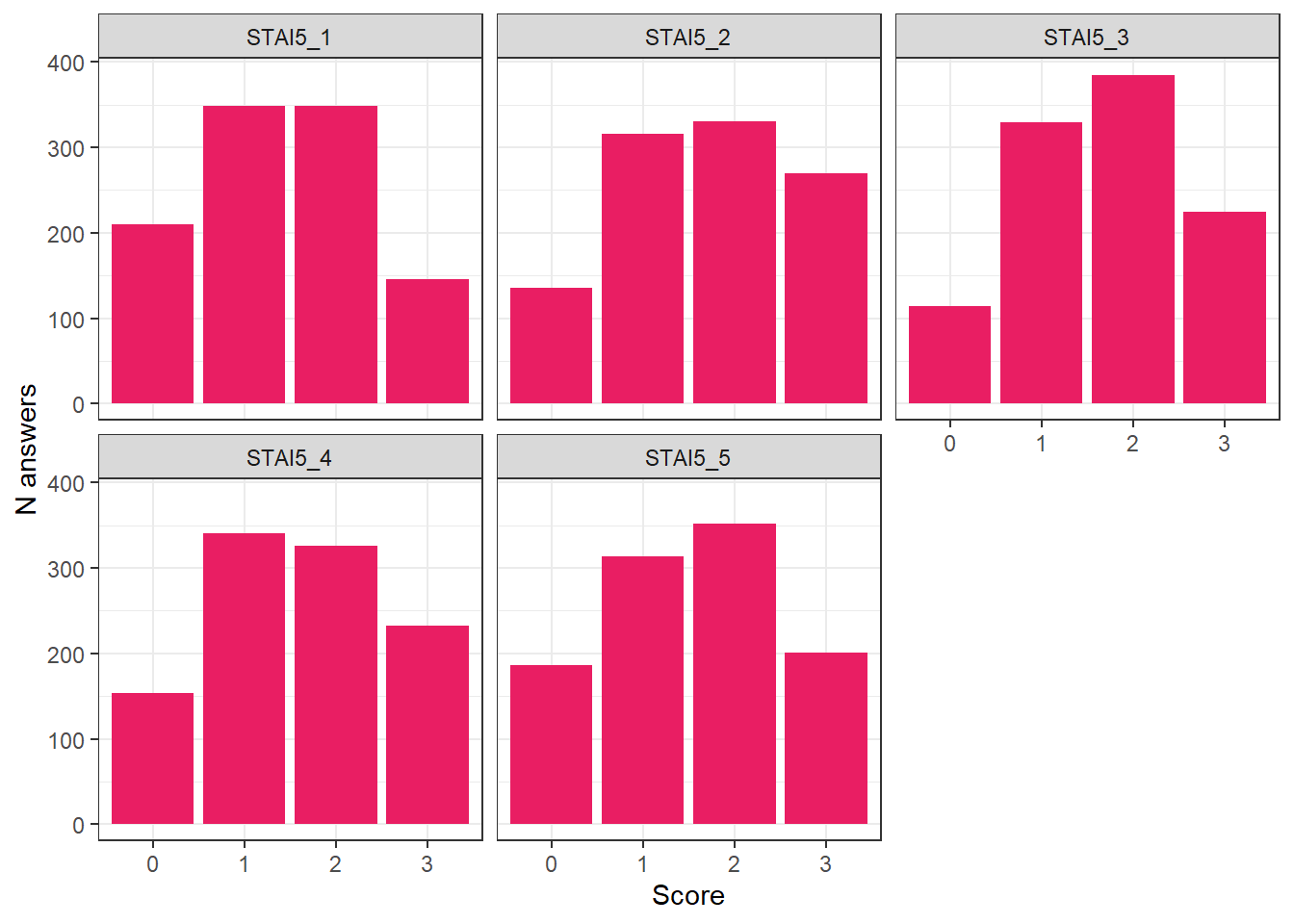

Code

df <- df |> 
  mutate(STAI5_General = (STAI5_1 + STAI5_2 + STAI5_3 + STAI5_4 + STAI5_5) / 5)

BDI-2

Code

df |>
  select(matches("BDI2_"), -BDI2_Duration, -BDI2_Order) |>
  pivot_longer(cols = matches("BDI2_"), names_to = "item", values_to = "score") |>
  ggplot(aes(x = as.factor(score))) +
  geom_bar(stat="count", fill="#2196F3") +
  facet_wrap(~item) +
  labs(x = "Score", y = "N answers") +
  theme_bw()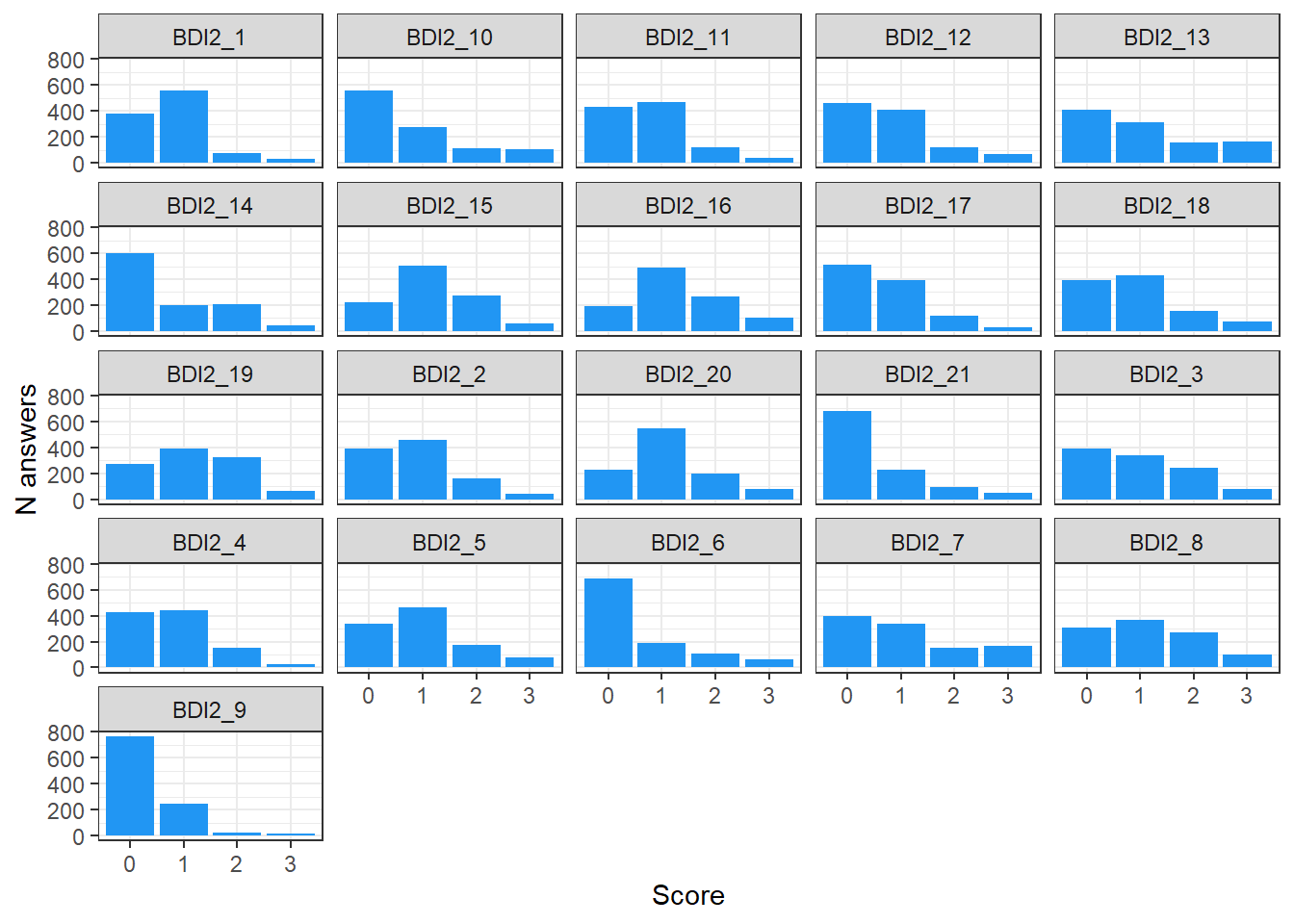

Code

df <- df |> 
  mutate(BDI2_Total = rowSums(select(df, matches("BDI2_"), -BDI2_Duration, -BDI2_Order)))

IAS

Code

df <- df |> 
  mutate(IAS_Total = rowSums(select(df, matches("IAS_"), -IAS_Duration, -IAS_Order)))

Exclusions

Code

outliers <- list()

Attention Checks

Only a subset of participants saw the version with attention checks.

Code

reject <- df |> 
  filter(!is.na(AttentionCheck_2)) |>
  select(Participant, Experimenter, starts_with("AttentionCheck")) |> 
  arrange(AttentionCheck_2, AttentionCheck_3) 

outliers$attentionchecks <- reject[reject$AttentionCheck_2 == 0 | reject$AttentionCheck_3 < 0.95, "Participant"]
outliers$attentionchecks <- outliers$attentionchecks[!is.na(outliers$attentionchecks)]
df$AttentionCheck <- ifelse(df$Participant %in% outliers$attentionchecks, "Failed", "Passed")

reject |> 
  gt::gt() |> 
  gt::data_color(columns = c("AttentionCheck_2", "AttentionCheck_3"), palette=c("red", "green")) |> 
  gt::data_color(columns = "Participant", fn=\(x) ifelse(x %in% outliers$attentionchecks, "red", "white")) |> 
  gt::opt_interactive(use_compact_mode = TRUE)

We removed 194 (18.42%) participants for failing the attention checks.

Code

dat <- mutate(df, Failed = ifelse(Participant %in% outliers$attentionchecks, 1, 0)) |> 
  filter(Gender %in% c("Female", "Male")) |> 
  filter(Experiment_Duration < 30) |> 
  mutate(Gender = as.factor(Gender)) |> 
  select(Failed, Gender, Experiment_Duration, Age, Ethnicity) 

m <- glm(Failed ~ Gender / Age, data=dat, family="binomial") 
parameters::parameters(m)

modelbased::estimate_relation(m, length=50) |> 
  ggplot(aes(x=Age, y=Predicted, color=Gender)) +
  geom_line()

Duration

Code

m <- mgcv::gam(Failed ~ s(Experiment_Duration), 
          data=df |> 
            filter(Experiment_Duration < 30) |> 
            mutate(Failed = ifelse(AttentionCheck == "Failed", 1, 0)), 
          family="binomial")

parameters::parameters(m)

# Fixed Effects

Parameter   | Log-Odds |   SE |         95% CI |      z |      df |      p
--------------------------------------------------------------------------
(Intercept) |    -1.52 | 0.08 | [-1.68, -1.36] | -18.46 | 1004.00 | < .001

# Smooth Terms

Parameter                         |    z |   df |     p
-------------------------------------------------------
Smooth term (Experiment Duration) | 2.84 | 1.00 | 0.092


The model has a log- or logit-link. Consider using `exponentiate =
  TRUE` to interpret coefficients as ratios.

Code

plot(estimate_relation(m, length=40))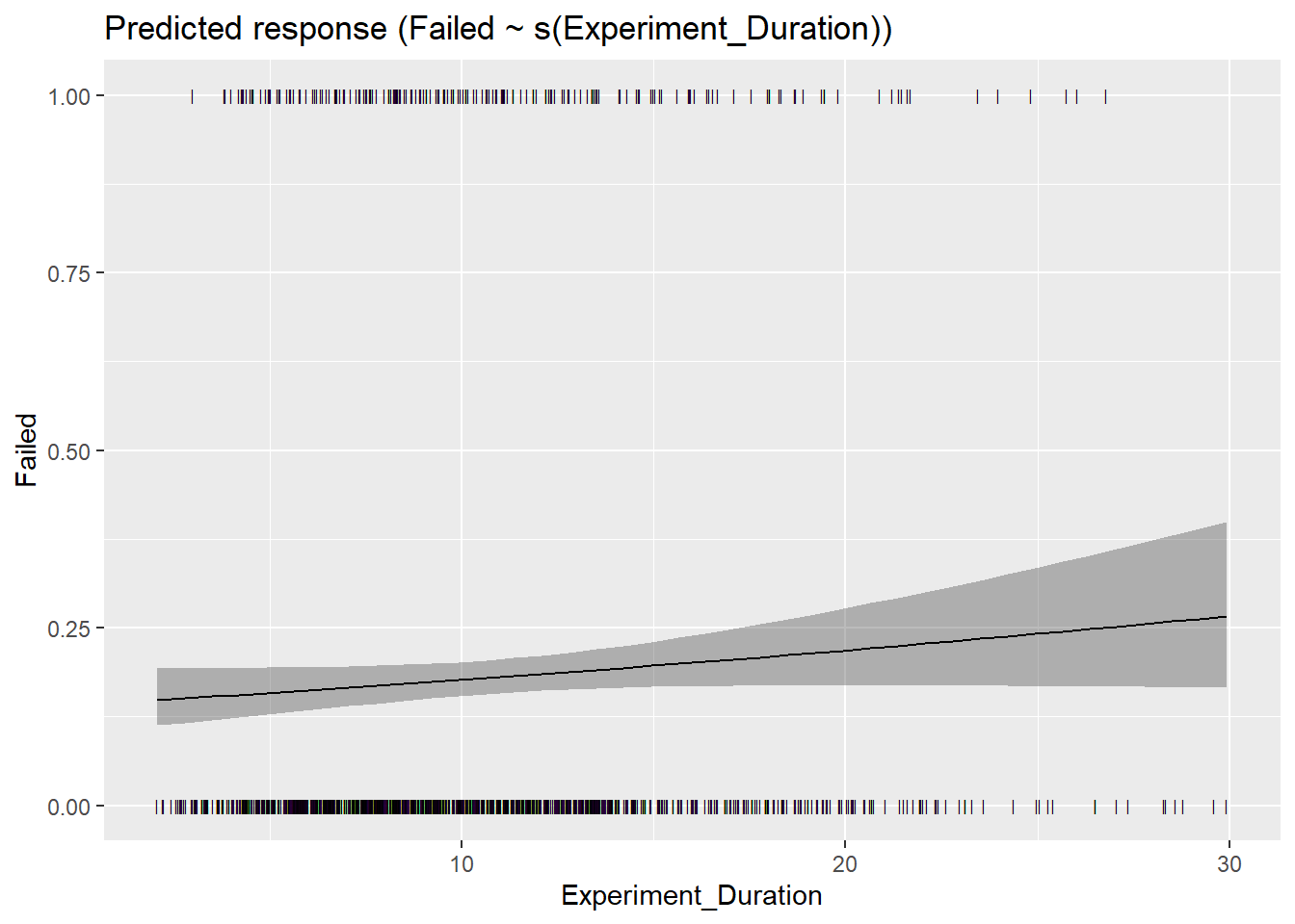

Code

df |> 
  filter(Experiment_Duration < 30) |> 
  select(Participant, Experiment_Duration, AttentionCheck) |> 
  mutate(Participant = fct_reorder(Participant, Experiment_Duration)) |>
  ggplot(aes(x=Participant, y=Experiment_Duration, fill=AttentionCheck)) +
  geom_bar(stat="identity") +
  theme_minimal() +
  theme(axis.text.x = element_blank())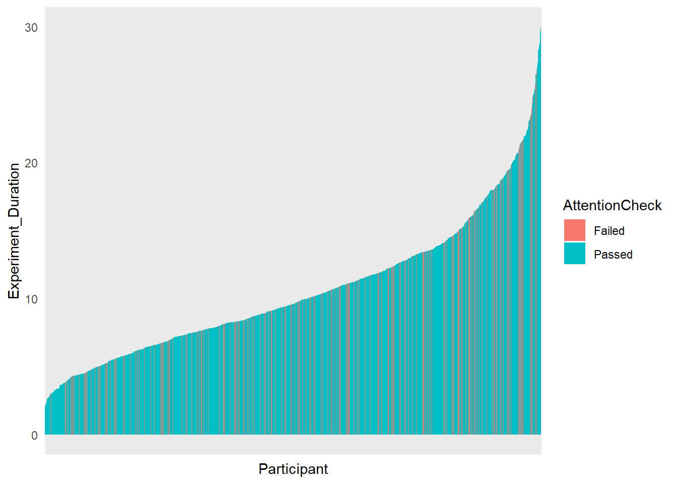

Response Coherence and Variability

Code

SD_per_dim <- function(x, dims="") {
  m <- matrix(nrow=nrow(x), ncol=0)
  for(s in dims) {
    m <- cbind(m, sapply(as.data.frame(t(x[grepl(s, names(x))])), sd))
  }
  m
}

df$BDI2_SD <- select(df, matches("BDI2_"), -BDI2_Duration, -BDI2_Order, -BDI2_Total) |> 
  SD_per_dim(dims=c("BDI2_")) |> 
  rowMeans()
df$STAI5_SD <- select(df, matches("STAI5_"), -STAI5_Duration, -STAI5_Order, -STAI5_General) |> 
  SD_per_dim(dims=c("STAI5_")) |> 
  rowMeans()
df$IAS_SD <- select(df, matches("IAS_"), -IAS_Duration, -IAS_Order, -IAS_Total) |> 
  SD_per_dim(dims=c("IAS_")) |> 
  rowMeans()

Code

m <- mgcv::gam(Failed ~ s(IAS_SD), 
          data=mutate(df, Failed = ifelse(AttentionCheck == "Failed", 1, 0)), 
          family="binomial") 
parameters::parameters(m)

# Fixed Effects

Parameter   | Log-Odds |   SE |         95% CI |      z |      df |      p
--------------------------------------------------------------------------
(Intercept) |    -1.51 | 0.08 | [-1.67, -1.35] | -18.63 | 1051.00 | < .001

# Smooth Terms

Parameter            |     z |   df |      p
--------------------------------------------
Smooth term (IAS SD) | 11.84 | 1.00 | < .001

Code

estimate_relation(m, length=40) |> 
  ggplot(aes(x=IAS_SD, y=Predicted)) +
  geom_ribbon(aes(ymin=CI_low, ymax=CI_high), alpha=0.2) +
  geom_line() + 
  ggside::geom_xsidedensity(data=df, aes(fill=AttentionCheck), alpha=0.3, color=NA)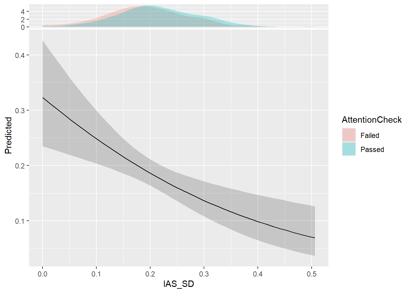

Code

df |> 
  select(Participant, IAS_SD, AttentionCheck) |> 
  mutate(Participant = fct_reorder(Participant, IAS_SD)) |>
  ggplot(aes(x=Participant, y=IAS_SD, fill=AttentionCheck)) +
  geom_bar(stat="identity") +
  theme_minimal() +
  theme(axis.text.x = element_blank())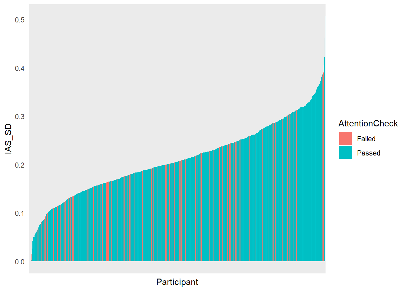

Code

outliers$ias_sd <- as.character(df[abs(standardize(df$IAS_SD, robust=TRUE)) > qnorm(0.995), "Participant"])
outliers$ias_sd <- outliers$ias_sd[!outliers$ias_sd %in% c(outliers$attentionchecks, outliers$duration)]

We removed 12 (1.14%) participants for failing being an outlier on the IAS’ SD value.

Multivariate Distance

Code

dfoutlier <- df |> 
  select(contains("IAS_"), -IAS_Duration, -IAS_Order, -IAS_Total, -IAS_SD) |>
  # select(contains("BDI2_"), -BDI2_Duration, -BDI2_Order, -BDI2_Total, -BDI2_SD) |>
  # select(contains("STAI5_"), -STAI5_Duration, -STAI5_Order, -STAI5_General, -STAI5_SD) |>
  # select(contains("MAIA2_"), -MAIA_Duration, -MAIA_Order) |>
  # datawizard::remove_empty_rows() |> 
  performance::check_outliers(
    method=c("optics", "mahalanobis_robust"),
    threshold=list(optics=2, optics_xi=0.1)) |> 
  as.data.frame() |> 
  mutate(Participant = fct_reorder(df$Participant, Distance_OPTICS),
         Outlier_AttentionCheck = ifelse(Participant %in% outliers$attentionchecks, 1, 0),
         Outlier_Distance = ifelse(abs(standardize(Distance_OPTICS, robust=TRUE)) > qnorm(0.995), 1, 0),
         Experiment_Duration = df$Experiment_Duration,
         Outlier = ifelse(Outlier_AttentionCheck == 1, "Failed Attention Checks", "Passed"))


outliers$distance <- as.character(dfoutlier[dfoutlier$Outlier_Distance == 1, "Participant"])
outliers$distance <- outliers$distance[!outliers$distance %in% c(outliers$attentionchecks, outliers$duration, outliers$ias_sd)]

m <- mgcv::gam(Outlier_AttentionCheck ~ s(Distance_OPTICS), data = dfoutlier, family = "binomial")
parameters::parameters(m)

# Fixed Effects

Parameter   | Log-Odds |   SE |         95% CI |      z |      df |      p
--------------------------------------------------------------------------
(Intercept) |    -1.50 | 0.08 | [-1.66, -1.34] | -18.67 | 1051.00 | < .001

# Smooth Terms

Parameter                     |    z |   df |     p
---------------------------------------------------
Smooth term (Distance OPTICS) | 7.05 | 1.00 | 0.008

Code

estimate_relation(m, length=40) |> 
  ggplot(aes(x=Distance_OPTICS, y=Predicted)) +
  geom_ribbon(aes(ymin=CI_low, ymax=CI_high), alpha=0.2) +
  geom_line() + 
  ggside::geom_xsidedensity(data=dfoutlier, aes(fill=Outlier), alpha=0.3, color=NA)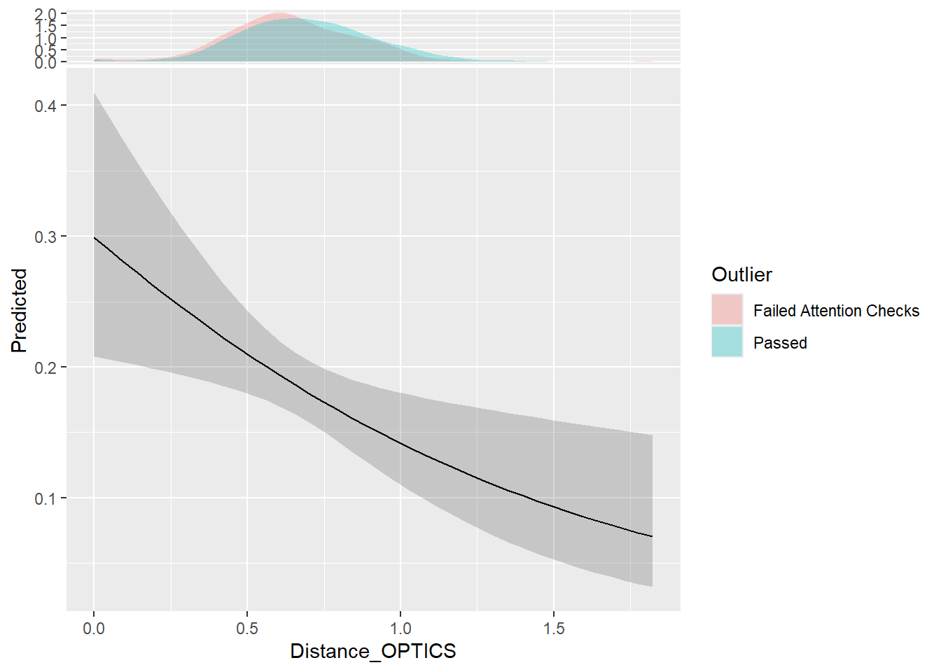

Code

dfoutlier |> 
  ggplot(aes(x=Participant, y=Distance_OPTICS, fill=Outlier)) +
  geom_bar(stat="identity") +
  theme_minimal() +
  theme(axis.text.x = element_blank())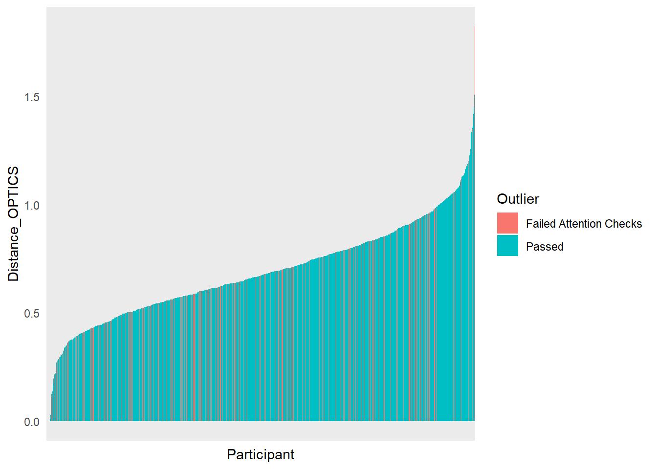

We removed 11 (1.04%) participants based on their multivariate distance. 23 (2.18%) outliers in total.

Code

# length(c(outliers$ias_sd, outliers$distance))
# insight::format_percent(length(c(outliers$ias_sd, outliers$distance)) / nrow(df))

df <- filter(df, !Participant %in% c(outliers$attentionchecks, outliers$ias_sd, outliers$distance))
df <- select(df, -starts_with("AttentionCheck"))

Final Sample

Participants

The final sample includes 836 participants (Mean age = 25.1, SD = 11.3, range: [18, 76], 0.1% missing; Gender: 73.8% women, 22.6% men, 2.87% non-binary, 0.72% missing; Education: Bachelor, 22.85%; Doctorate, 2.15%; High School, 63.52%; Master, 6.22%; missing, 0.24%; Other, 5.02%).

Age

Code

p_age <- df |>  
  mutate(Gender = ifelse(is.na(Gender), "Missing", Gender)) |>
  ggplot(aes(x = x)) +
  geom_histogram(aes(x = Age, fill=Gender), bins=28) +
  geom_vline(xintercept = mean(df$Age), color = "red", linewidth=1.5) +
  # geom_label(data = data.frame(x = mean(df$Age) * 1.15, y = 0.95 * 75), aes(y = y), color = "red", label = paste0("Mean = ", format_value(mean(df$Age)))) +
  scale_fill_manual(values = c("Male"= "#64B5F6", "Female"= "#F06292", "Other"="orange", "Missing"="brown")) +
  scale_x_continuous(expand = c(0, 0)) +
  scale_y_continuous(expand = c(0, 0)) +
  labs(title = "Age", y = "Number of Participants", color = NULL, subtitle = "Distribution of participants' age") +
  theme_modern(axis.title.space = 10) +
  theme(
    plot.title = element_text(size = rel(1.2), face = "bold", hjust = 0),
    plot.subtitle = element_text(size = rel(1.2), vjust = 7),
    axis.text.y = element_text(size = rel(1.1)),
    axis.text.x = element_text(size = rel(1.1)),
    axis.title.x = element_blank()
  )
p_age

Warning: Removed 1 row containing non-finite outside the scale range
(`stat_bin()`).

Warning: Removed 1 row containing missing values or values outside the scale range
(`geom_vline()`).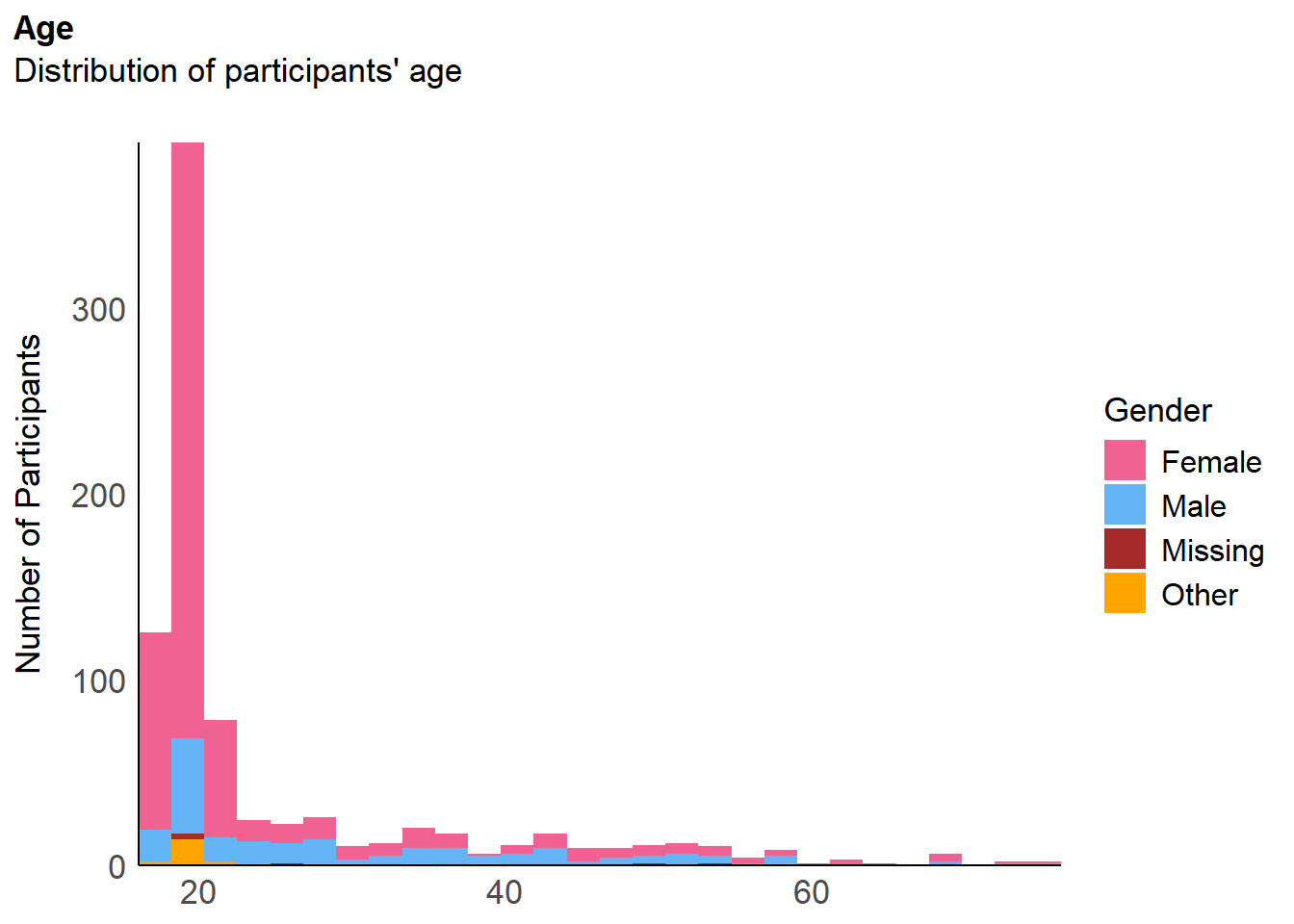

Education

Code

p_edu <- df |>
  mutate(
    Education = ifelse(Education == "", NA, Education),
    Education = fct_relevel(Education, "Other", "High School", "Bachelor", "Master", "Doctorate")) |> 
  ggplot(aes(x = Education)) +
  geom_bar(aes(fill = Education)) +
  scale_y_continuous(expand = c(0, 0), breaks= scales::pretty_breaks()) +
  scale_fill_viridis_d(guide = "none") +
  labs(title = "Education", y = "Number of Participants", subtitle = "Participants per achieved education level") +
  theme_modern(axis.title.space = 15) +
  theme(
    plot.title = element_text(size = rel(1.2), face = "bold", hjust = 0),
    plot.subtitle = element_text(size = rel(1.2), vjust = 7),
    axis.text.y = element_text(size = rel(1.1)),
    axis.text.x = element_text(size = rel(1.1)),
    axis.title.x = element_blank()
  )
p_edu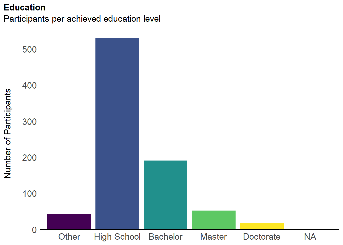

Table 1

Code

df$PHQ4_Duration[df$PHQ4_Duration > 3] <- NA

table1 <- df |> 
  select(Age, 
         PHQ4_Condition, 
         PHQ4_Total,
         PHQ4_Duration,
         STAI5_General,
         BDI2_Total) |> 
  report::report_sample(by = "PHQ4_Condition")

table1$Variable <- str_remove_all(table1$Variable, fixed("Mean "))
table1$Variable <- str_remove_all(table1$Variable, fixed(" (SD)"))
table1$Variable <- c("Age", "PHQ4 (Total)", "PHQ4 (Duration)", "STAI5", "BDI2")

Code

add_bf <- function(df, var="PHQ4_Duration") {
  dat <- df[, c(var, "PHQ4_Condition")]
  dat <- dat[complete.cases(dat), ]
  r <- report::report(t.test(dat[[var]] ~ dat[["PHQ4_Condition"]]), verbose=FALSE)
  x <- as.data.frame(r)
  f <- as.formula(paste(var, "~ PHQ4_Condition"))
  x$BF <- as.data.frame(BayesFactor::ttestBF(formula=f, data=dat))$bf
  x$Parameter <- var
  x
}


table1_inference <- rbind(
  add_bf(filter(df, !is.na(Age)), "Age"),
  add_bf(df, var="PHQ4_Total"),
  add_bf(df, var="PHQ4_Duration"),
  add_bf(df, "STAI5_General"),
  add_bf(df, "BDI2_Total")
) |> 
  select(Parameter, t, df_error, p, BF) |> 
  mutate(Parameter = str_remove_all(Parameter, fixed("df$")))

table1$BF <- table1_inference$BF
insight::display(table1)

Descriptive Statistics
Variable	PHQ4 - Original (n=396)	PHQ4 - Revised (n=440)	Total (n=836)	BF
Age	25.48 (11.69)	24.69 (10.91)	25.07 (11.29)	0.13
PHQ4 (Total)	4.70 (3.00)	4.45 (3.00)	4.57 (3.00)	0.16
PHQ4 (Duration)	0.40 (0.30)	0.40 (0.28)	0.40 (0.29)	0.08
STAI5	1.57 (0.77)	1.55 (0.77)	1.56 (0.77)	0.08
BDI2	18.74 (11.84)	17.63 (11.13)	18.16 (11.47)	0.20

Distributions

Code

df |> 
  select(PHQ4_Condition, 
         STAI5 = STAI5_General,
         BDI2 = BDI2_Total,
         PHQ4_Total) |> 
  standardize() |> 
  estimate_density(by = "PHQ4_Condition", method="KernSmooth") |> 
  ggplot(aes(x=x, y=y)) +
  geom_line(aes(color = Parameter), linewidth=2) +
  scale_color_manual(values = c("STAI5" = "#E91E63", "BDI2" = "#2196F3", "PHQ4_Total" = "#9C27B0")) +
  labs(x = "Standardized Score", y = "Distribution") +
  facet_wrap(~PHQ4_Condition) +
  theme_bw()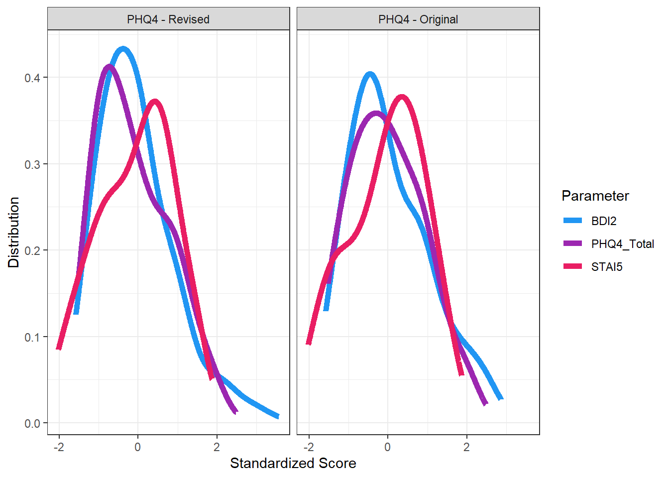

Mood Disorders

Diagnostic

Code

p1 <- select(df, Participant, Gender, starts_with("Disorder_")) |> 
  pivot_longer(cols = starts_with("Disorder_"), names_to = "Disorder", values_to = "Value") |> 
  mutate(Disorder = str_remove_all(Disorder, fixed("Disorder_"))) |> 
  summarize(N = sum(Value) / nrow(df), .by=c("Gender", "Disorder")) |> 
  mutate(N_tot = sum(N), .by="Disorder") |>
  mutate(Disorder = fct_reorder(Disorder, desc(N_tot))) |>
  ggplot(aes(x = Disorder, y = N, fill=Gender)) +
  geom_bar(stat = "identity") +
  scale_fill_manual(values = c("Male"= "#64B5F6", "Female"= "#F06292", "Other"="orange", "Missing"="brown")) +
  scale_y_continuous(expand = c(0, 0), labels=scales::percent) +
  labs(title = "Mood Disorders", y = "Number of Participants", subtitle = "Participants per self-declared mood disorder", x="Type") +
  theme(axis.text.x = element_text(angle = 45, hjust = 1)) +
  theme_minimal()

p2 <- select(df, Participant, Gender, starts_with("DisorderTreatment_")) |> 
  pivot_longer(cols = starts_with("DisorderTreatment_"), names_to = "Treatment", values_to = "Value") |> 
  mutate(Treatment = str_remove_all(Treatment, fixed("DisorderTreatment_"))) |> 
  summarize(N = sum(Value) / nrow(df), .by=c("Gender", "Treatment")) |> 
  mutate(N_tot = sum(N), .by="Treatment") |>
  mutate(Treatment = fct_reorder(Treatment, desc(N_tot))) |>
  ggplot(aes(x = Treatment, y = N, fill=Gender)) +
  geom_bar(stat = "identity") +
  scale_fill_manual(values = c("Male"= "#64B5F6", "Female"= "#F06292", "Other"="orange", "Missing"="brown")) +
  scale_y_continuous(expand = c(0, 0), labels=scales::percent) +
  labs(title = "Treatment", y = "Number of Participants", subtitle = "Participants per treatment", x="Type") +
  theme(axis.text.x = element_text(angle = 45, hjust = 1)) +
  theme_minimal()

p1 / p2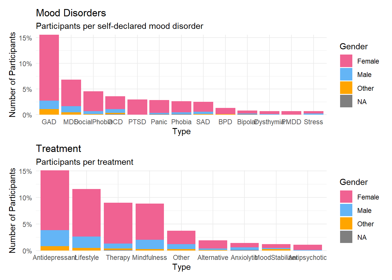

Code

df$MoodDisorder <- rowSums(select(df, DisorderTreatment_MoodStabilizer, DisorderTreatment_Antidepressant, DisorderTreatment_Anxiolytic))
df$MoodDisorder <- ifelse(df$MoodDisorder > 0, TRUE, FALSE)

df$Treatment <- rowSums(select(df, DisorderTreatment_MoodStabilizer, DisorderTreatment_Antidepressant, DisorderTreatment_Anxiolytic, DisorderTreatment_Therapy))
df$Treatment <- ifelse(df$Treatment > 0, TRUE, FALSE)

df$Depression <- rowSums(select(df, Disorder_MDD, Disorder_Dysthymia))
df$Depression <- ifelse(df$Depression > 0 & df$Treatment, TRUE, FALSE)

df$Anxiety <- rowSums(select(df, Disorder_GAD, Disorder_Panic))
df$Anxiety <- ifelse(df$Anxiety > 0 & df$Treatment, TRUE, FALSE)

df$DisorderHistory <- ifelse(df$DisorderHistory == "Yes", TRUE, FALSE)

136 participants (16.27%) have a mood disorder, as indexed by the use of a mood stabilizer, antidepressant, or anxiolytic treatment.
51 participants (6.10%) were labelled as having Depression, as indexed by the self-reported presence of MDD together with the the use of a treatment (antidepressent, anxiolytic and/or therapy).
87 participants (10.41%) were labelled as having Anxiety, as indexed by the self-reported presence of GAD or Panic Disorder together with the the use of a treatment (antidepressent, anxiolytic and/or therapy).
191 participants (22.85%) reported having a history of mood disorder.

Save

write.csv(df, "../data/data.csv", row.names = FALSE)