PHQ4R - Data Analysis (Study 2)

Data Preparation

Code

library(tidyverse)
library(easystats)
library(patchwork)
library(ggside)
library(ggdist)
library(mirt)

Code

df <- read.csv("../data/data.csv") |> 
  mutate(
    PHQ4_Condition = fct_relevel(PHQ4_Condition, "PHQ4 - Original"),
    PHQ4_Condition = fct_recode(PHQ4_Condition, "Original" = "PHQ4 - Original", "Revised" = "PHQ4 - Revised"),
    # BDI2_Category = ifelse(BDI2_Total <= 12, "Subclinical", ifelse(BDI2_Total <= 18, "Mild", "Moderate+")),
    BDI2_Category = ifelse(BDI2_Total <= 18, "Minimal - Mild", "Moderate - Severe"),
    STAI5_Category = ifelse(STAI5_General < 2, "Minimal - Mild", "Moderate - Severe"),
    PHQ4_Depression_Fac = as.factor(PHQ4_Depression)
  )

colors <- c("Original" = "#607D8B", "Revised" = "#FF9800")

Depression

Relationship with BDI-2

Code

model <- lm(BDI2_Total ~ PHQ4_Depression * PHQ4_Condition, data = df)

parameters::parameters(model) |> 
  display()

Parameter	Coefficient	SE	95% CI	t(832)	p
(Intercept)	8.23	0.59	(7.08, 9.39)	13.96	< .001
PHQ4 Depression	5.34	0.23	(4.90, 5.79)	23.51	< .001
PHQ4 Condition (Revised)	-0.13	0.82	(-1.73, 1.47)	-0.16	0.871
PHQ4 Depression × PHQ4 Condition (Revised)	-0.05	0.33	(-0.70, 0.60)	-0.15	0.883

Code

get_bf <- function(resp="BDI2_Total", pred="PHQ4_Depression", levels=c(0, 0.5)) {
  if(length(levels) == 2) {
    bf <- BayesFactor::ttestBF(
      df[df[[pred]] == levels[1] & df$PHQ4_Condition=="Revised", resp], 
      df[df[[pred]] == levels[2] & df$PHQ4_Condition=="Revised", resp])
  } else {
    bf <- BayesFactor::ttestBF(
      df[df[[pred]]==levels & df$PHQ4_Condition=="Original", resp],
      df[df[[pred]]==levels & df$PHQ4_Condition=="Revised", resp])
  }
  insight::format_bf(exp(bf@bayesFactor$bf), stars=TRUE)
}

get_databf <- function(resp="BDI2_Total", pred="PHQ4_Depression", y1, y2) {
  
  # Between scores comparisons
  bfs <- data.frame(
    BF = c(get_bf(resp, pred, c(0, 0.5)), 
           get_bf(resp, pred, c(0.5, 1)), 
           get_bf(resp, pred, c(1, 1.5)), 
           get_bf(resp, pred, c(1.5, 2)),
           get_bf(resp, pred, c(2, 2.5)),
           get_bf(resp, pred, c(2.5, 3)))
  )
  bfs[[pred]] <- c(0.25, 0.75, 1.25, 1.75, 2.25, 2.75)
  bfs[[resp]] <- y1
  bfs$color <- "Revised"
  
  # Within scores comparisons
  bfs2 <- data.frame(
    BF = c(get_bf(resp, pred, 0), 
           get_bf(resp, pred, 1), 
           get_bf(resp, pred, 2),
           get_bf(resp, pred, 3),
           get_bf(resp, pred, 4))
  )
  bfs2[[pred]] <- c(0, 1, 2, 3, 4)
  bfs2[[resp]] <- y2
  bfs2$color <- "Original"
  
  bf <- rbind(bfs, bfs2)
  
  # Lines behing labels
  lines <- data.frame(
    xmin = c(0, 0.5, 1, 1.5, 2, 2.5),
    xmax = c(0.5, 1, 1.5, 2, 2.5, 3),
    y = y1
  )
  
  list(bf=bf, lines=lines)
}


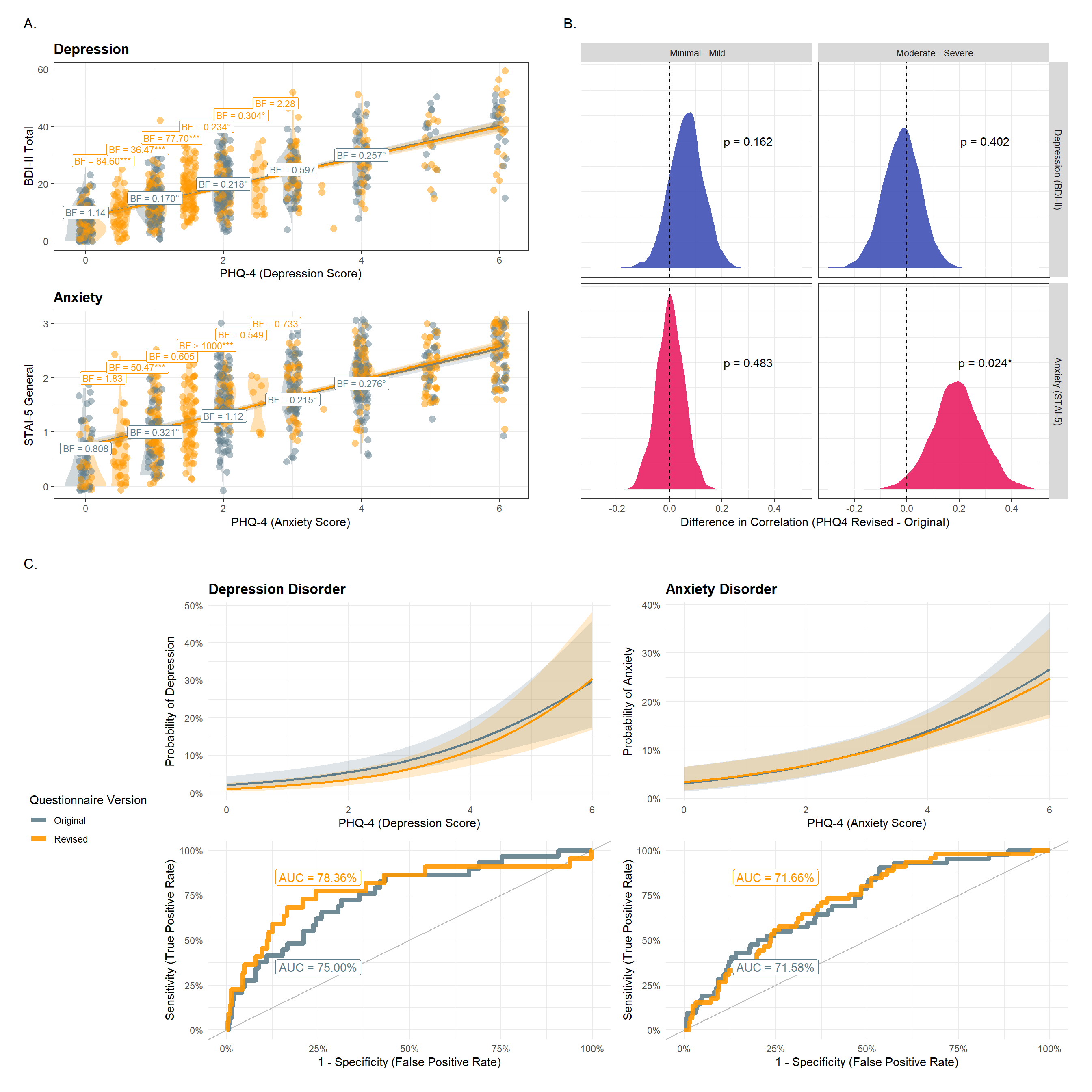
bfs <- get_databf(resp="BDI2_Total", pred="PHQ4_Depression", y1=c(28, 32, 36, 40, 44, 48), y2=c(10, 15, 20, 25, 30))

p_dep <- df |> 
  ggplot(aes(x = PHQ4_Depression, y = BDI2_Total), width=0.1) +
  ggdist::stat_slab(
    data = df[df$PHQ4_Condition == "Original" & df$PHQ4_Depression <= 4, ], 
    fill = colors["Original"],
    alpha=0.3,
    scale = 0.3,
    position = position_dodge(width = 1),
    side = "left") +
  ggdist::stat_slab(
    data = df[df$PHQ4_Condition == "Revised" & df$PHQ4_Depression %in% c(0, 1, 2, 3, 4), ], 
    fill = colors["Revised"],
    alpha=0.3,
    scale = 0.3,
    position = position_dodge(width = 1),
    side = "right") +
  ggdist::stat_slab(
    data = df[df$PHQ4_Depression %in% c(0.5, 1.5, 2.5), ], 
    fill = colors["Revised"],
    alpha=0.3,
    scale = 0.3,
    position = position_dodge(width = 1),
    side = "both") +
  geom_jitter2(aes(color = PHQ4_Condition), width=0.1, alpha=0.5, size=3) +
  geom_smooth(aes(color = PHQ4_Condition, fill=PHQ4_Condition), 
              method = "lm", formula="y~x", alpha=0.2, key_glyph = draw_key_rect) +
  geom_segment(data=bfs$lines, aes(x=xmin, xend=xmax, y=y, yend=y), color=colors["Revised"], linewidth=0.5) +
  geom_label(data = bfs$bf, aes(x = PHQ4_Depression, y = BDI2_Total, label = BF, color=color), size=3) +
  scale_fill_manual(values = colors) +
  scale_color_manual(values = colors) +
  theme_bw() +
  # ggside::geom_xsidedensity(aes(fill = PHQ4_Condition), color=NA, alpha=0.5) +
  ggside::scale_xsidey_continuous(expand = c(0, 0)) +
  # ggside::geom_ysidedensity(aes(fill = PHQ4_Condition), color=NA, alpha=0.5) +
  ggside::scale_ysidex_continuous(expand = c(0, 0)) +
  ggside::theme_ggside_void() +
  coord_cartesian(xlim=c(-0.15, 6.1)) +
  guides(color="none", fill=guide_legend(override.aes = list(alpha=1))) +
  labs(
    x = "PHQ-4 (Depression Score)",
    y = "BDI-II Total",
    color = "PHQ4 Version",
    fill = "PHQ4 Questionnaire Version",
    title="Depression",
  ) +
  theme(legend.position = "top",
        plot.title = element_text(face="bold"))
p_dep

Warning: `is.ggproto()` was deprecated in ggplot2 3.5.2.
ℹ Please use `is_ggproto()` instead.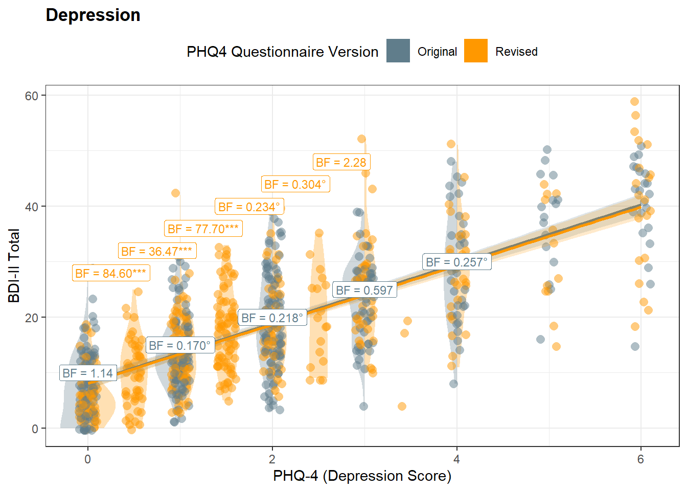

Predictive Performance

Code

m <- glm(Depression ~ PHQ4_Depression * PHQ4_Condition, data = df, family="binomial")

display(parameters::parameters(m))

Parameter	Log-Odds	SE	95% CI	z	p
(Intercept)	-3.84	0.40	(-4.70, -3.11)	-9.52	< .001
PHQ4 Depression	0.50	0.11	(0.29, 0.71)	4.64	< .001
PHQ4 Condition (Revised)	-0.70	0.62	(-1.95, 0.51)	-1.12	0.262
PHQ4 Depression × PHQ4 Condition (Revised)	0.12	0.16	(-0.20, 0.44)	0.75	0.454

Code

p_mdd <- m |> 
  estimate_relation(length=20) |> 
  ggplot(aes(x=PHQ4_Depression, y=Predicted)) +
  geom_ribbon(aes(ymin=CI_low, ymax=CI_high, fill=PHQ4_Condition), alpha=0.2) +
  geom_line(aes(color=PHQ4_Condition), linewidth=1) +
  scale_fill_manual(values = colors) +
  scale_color_manual(values = colors) +
  scale_y_continuous(labels=scales::percent) +
  labs(y = "Probability of Depression",
       x= "PHQ-4 (Depression Score)",
       title = "Depression Disorder",
       fill = "Questionnaire Version",
       color = "Questionnaire Version") +
  theme_minimal()  +
  theme(plot.title = element_text(face="bold"),
        legend.position = "none")

Code

make_roc <- function(m) {
  resp <- insight::find_response(m)
  pred <- insight::find_predictors(m)
  f <- as.formula(paste0(resp, " ~ ", pred$conditional[1]))
  m1 <- glm(f, data = df[df$PHQ4_Condition == "Original", ], family="binomial") 
  m2 <- glm(f, data = df[df$PHQ4_Condition == "Revised", ], family="binomial")
  
  roc1 <- performance_roc(m1) 
  roc2 <- performance_roc(m2)
  rocs <- data.frame(AUC = c(
    bayestestR::area_under_curve(roc1$Specificity, roc1$Sensitivity),
    bayestestR::area_under_curve(roc2$Specificity, roc2$Sensitivity)),
    PHQ4_Condition = c("Original", "Revised"))
  rocs$AUC <- paste0("AUC = ", insight::format_percent(rocs$AUC))
  rocs$x <- c(0.25, 0.25)
  rocs$y <- c(0.35, 0.85)
  
  rbind(
    mutate(as.data.frame(roc1), PHQ4_Condition = "Original"),
    mutate(as.data.frame(roc2), PHQ4_Condition = "Revised")
  ) |> 
    ggplot(aes(x=Specificity)) +
    geom_abline(intercept=0, slope=1, color="gray") +
    geom_line(aes(y=Sensitivity, color=PHQ4_Condition), linewidth=2, alpha=0.9) +
    geom_label(data=rocs, aes(x=x, y=y, label=AUC), color=colors) +
    labs(x= "1 - Specificity (False Positive Rate)", y="Sensitivity (True Positive Rate)",
         color="Questionnaire Version") +
    scale_color_manual(values=colors) +
    scale_x_continuous(labels=scales::percent) +
    scale_y_continuous(labels=scales::percent) +
    theme_minimal()
}

p_mddroc <- make_roc(m)

Code

p_mdd / p_mddroc + plot_layout(guides="collect")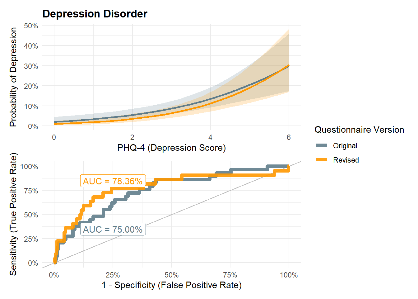

IRT

These completementary analyses were suggested during review to also apply IRT to the second sample. Additionally, we also computed “empirical coverage” curves.

Code

dat_irt <- df |> 
  filter(PHQ4_Condition == "Revised") |>
  select(starts_with("PHQ4"), BDI2_Total, STAI5_General) |> 
  mutate(Depression_3 = as.numeric(as.factor(PHQ4_Depression_3)),
         Depression_4 = as.numeric(as.factor(PHQ4_Depression_4)),
         Anxiety_1 = as.numeric(as.factor(PHQ4_Anxiety_1)),
         Anxiety_2 = as.numeric(as.factor(PHQ4_Anxiety_2)))

irt_model1 <- mirt::mirt(data = dat_irt[c("Depression_3", "Depression_4")],
                  itemtype = 'graded',
                  verbose = FALSE) 
irt_model2 <- mirt::mirt(data = dat_irt[c("Anxiety_1", "Anxiety_2")],
                         optimizer = "nlminb",
                  itemtype = 'graded',
                  verbose = FALSE) 

# plot(irt_model, type = "trace", theta_lim = c(-3, 3))

irt_data1  <- mirt::fscores(irt_model1, full.scores.SE = TRUE) |>
  as.data.frame() |> 
  mutate(Groundtruth = dat_irt$BDI2_Total,
         PHQ4_Score = dat_irt$PHQ4_Depression,
         Dimension = "Depression") 
irt_data2  <- mirt::fscores(irt_model2, full.scores.SE = TRUE) |>
  as.data.frame() |> 
  mutate(Groundtruth = dat_irt$STAI5_General,
         PHQ4_Score = dat_irt$PHQ4_Anxiety,
         Dimension = "Anxiety")

irt_data1$Label1 <- insight::format_value(cor(irt_data1$F1, irt_data1$Groundtruth))
irt_data1$Label2 <- insight::format_value(cor(irt_data1$F1, irt_data1$PHQ4_Score))
irt_data2$Label1 <- insight::format_value(cor(irt_data2$F1, irt_data2$Groundtruth))
irt_data2$Label2 <- insight::format_value(cor(irt_data2$F1, irt_data2$PHQ4_Score))

irt_data <- rbind(irt_data1, irt_data2) |> 
  mutate(Label1 = paste("r =", Label1),
         Label2 = paste("r =", Label2)) 

irt_data |> 
  ggplot() +
  geom_jitter(aes(x = F1, y = Groundtruth), width = 0.05, height = 0.05) +
  geom_smooth(aes(x = F1, y = Groundtruth), method = "lm", color = "red", formula = "y ~ x") +
  geom_text(data = dplyr::distinct(irt_data[c("Dimension", "Label1")]), aes(label = Label1),
    x = -1, y = c(55, 3), size = 5, color = "red"
  ) +
  facet_wrap(~ Dimension, scales = "free_y", ncol = 1) +
  labs(x = "Theta latent factor extracted from IRT", y = "Ground truth score (BDI-II or STAI-5)") +
  theme_minimal() |
  irt_data |> 
  ggplot() +
  geom_jitter(aes(x = F1, y = PHQ4_Score), width = 0.05, height = 0.05) +
  geom_smooth(aes(x = F1, y = PHQ4_Score), method = "lm", color = "blue", formula = "y ~ x", se = FALSE) +
  geom_smooth(aes(x = F1, y = PHQ4_Score), method = "lm", color = "darkorange", formula = "y ~ poly(x, 2)", se = FALSE) +
  geom_text(data = dplyr::distinct(irt_data[c("Dimension", "Label2")]), aes(label = Label2),
    x = -1, y = c(6, 6), size = 5, color = "red"
  ) +
  facet_wrap(~ Dimension, scales = "free_y", ncol = 1) +
  labs(x = "Theta latent factor extracted from IRT", y = "PHQ4 Score (Average)") +
  theme_minimal()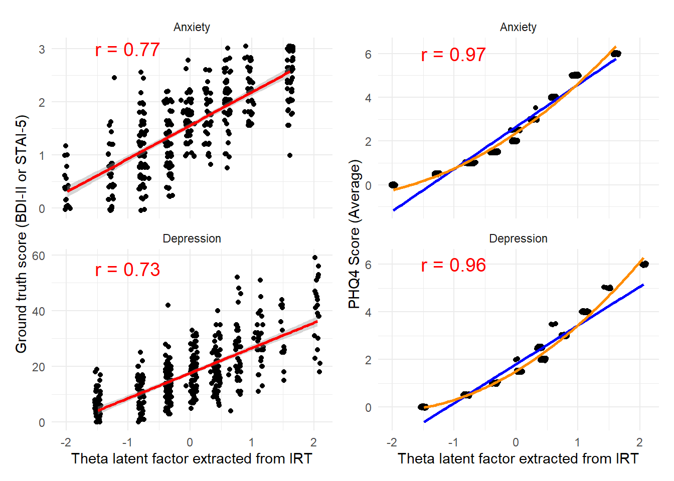

Code

add_labels <- function(x) {
  x <- case_when(
    x == 0 ~ "Not at all",
    x == 0.5 ~ "Once or twice",
    x == 1 ~ "Several days",
    x == 2 ~ "More than half the days",
    .default = "Nearly every day"
  )
  fct_relevel(x, c("Not at all", "Once or twice", "Several days", "More than half the days", "Nearly every day"))
}

rbind(
  mutate(dat_irt, 
         Item = "D1: Feeling down, depressed, or hopeless", 
         Response = add_labels(PHQ4_Depression_3),
         Outcome = BDI2_Total),
  mutate(dat_irt, 
         Item = "D2: Little interest or pleasure in doing things",
         Response = add_labels(PHQ4_Depression_4),
         Outcome = BDI2_Total),
  mutate(dat_irt, 
         Item = "A1: Feeling nervous, anxious, or on edge",
         Response = add_labels(PHQ4_Anxiety_1),
         Outcome = STAI5_General),
  mutate(dat_irt, 
         Item = "A2: Not being able to stop or control worrying",
         Response = add_labels(PHQ4_Anxiety_2),
         Outcome = STAI5_General)
  ) |>
  estimate_density(method = "KernSmooth", select = "Outcome", by = c("Item", "Response")) |> 
  ggplot(aes(x = x, y = y, color = Response)) +
  geom_line(linewidth = 1) +
  labs(x = "Ground truth measure (BDI or STAI)", y = "Distribution") +
  facet_wrap(~ Item, scales = "free") +
  scale_y_continuous(expand = expansion(add = c(0, 0.001))) +
  scale_x_continuous(expand = expansion(add = c(0, 0))) +
  see::scale_color_flat_d("rainbow") +
  see::theme_modern(axis.title.space = 5) +
  theme(strip.background = element_rect(fill = "#EEEEEE", colour = "white"),
        axis.text.y = element_blank())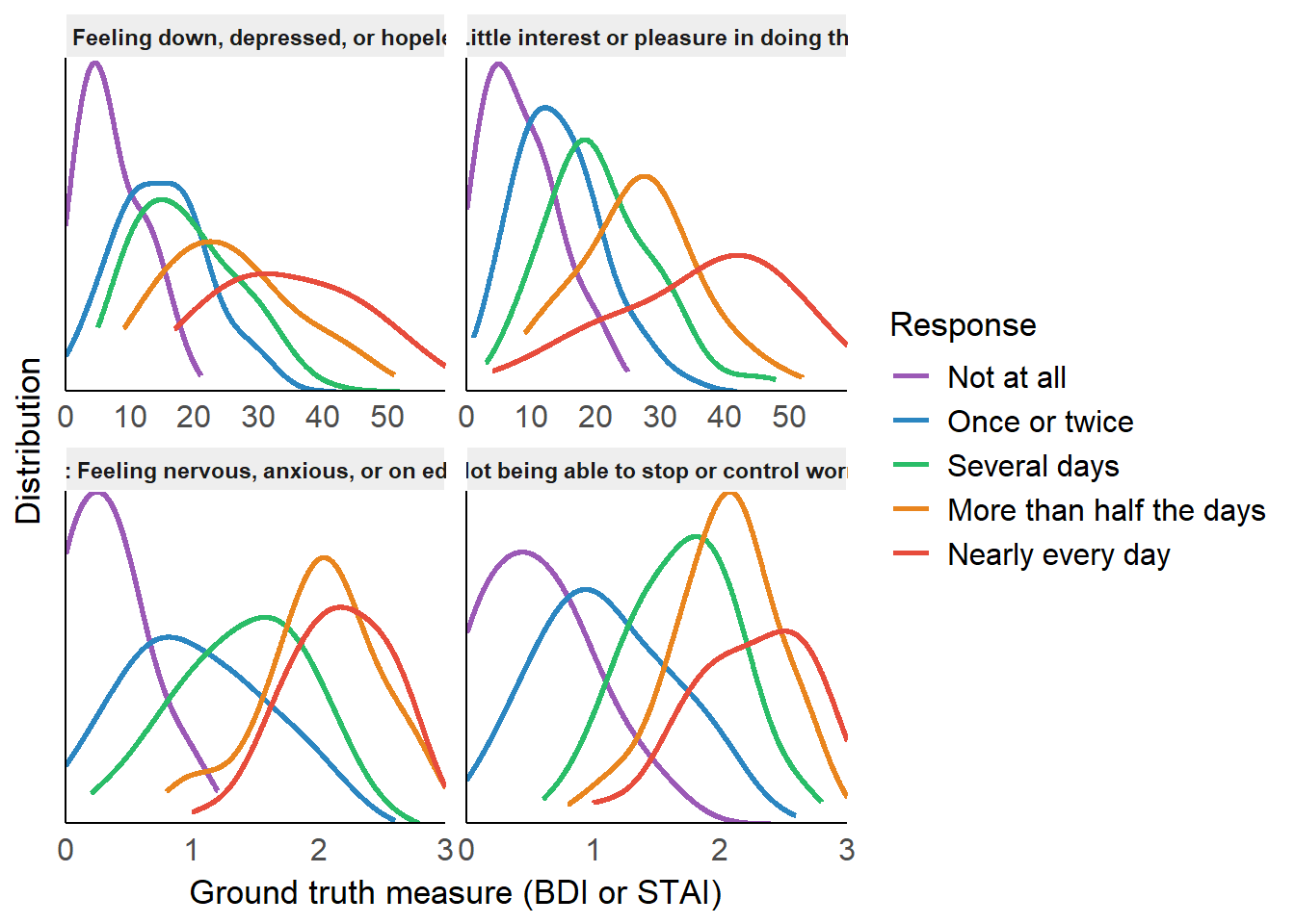

Anxiety

Relationship with STAI

Code

model <- lm(STAI5_General ~ PHQ4_Anxiety * PHQ4_Condition, data = df)

parameters::parameters(model) |> 
  display()

Parameter	Coefficient	SE	95% CI	t(832)	p
(Intercept)	0.76	0.05	(0.66, 0.85)	15.33	< .001
PHQ4 Anxiety	0.30	0.02	(0.27, 0.33)	19.72	< .001
PHQ4 Condition (Revised)	-0.02	0.07	(-0.15, 0.11)	-0.32	0.750
PHQ4 Anxiety × PHQ4 Condition (Revised)	0.01	0.02	(-0.03, 0.05)	0.56	0.576

Code

bfs <- get_databf(resp="STAI5_General", pred="PHQ4_Anxiety", y1=c(2.0, 2.2, 2.4, 2.6, 2.8, 3), y2=c(0.7, 1, 1.3, 1.6, 1.9))

p_anx <- df |> 
  ggplot(aes(x = PHQ4_Anxiety, y = STAI5_General), width=0.1) +
  ggdist::stat_slab(
    data = df[df$PHQ4_Condition == "Original" & df$PHQ4_Anxiety <= 4, ], 
    fill = colors["Original"],
    alpha=0.3,
    scale = 0.3,
    position = position_dodge(width = 1),
    side = "left") +
  ggdist::stat_slab(
    data = df[df$PHQ4_Condition == "Revised" & df$PHQ4_Anxiety %in% c(0, 1, 2, 3, 4), ], 
    fill = colors["Revised"],
    alpha=0.3,
    scale = 0.3,
    position = position_dodge(width = 1),
    side = "right") +
  ggdist::stat_slab(
    data = df[df$PHQ4_Anxiety %in% c(0.5, 1.5, 2.5), ], 
    fill = colors["Revised"],
    alpha=0.3,
    scale = 0.3,
    position = position_dodge(width = 1),
    side = "both") +
  geom_jitter2(aes(color = PHQ4_Condition), width=0.1, alpha=0.5, size=3) +
  geom_smooth(aes(color = PHQ4_Condition, fill=PHQ4_Condition), 
              method = "lm", formula="y~x", alpha=0.2, key_glyph = draw_key_rect) +
  geom_segment(data=bfs$lines, aes(x=xmin, xend=xmax, y=y, yend=y), color=colors["Revised"], linewidth=0.5) +
  geom_label(data = bfs$bf, aes(x = PHQ4_Anxiety, y = STAI5_General, label = BF, color=color), size=3) +
  scale_fill_manual(values = colors) +
  scale_color_manual(values = colors) +
  theme_bw() +
  # ggside::geom_xsidedensity(aes(fill = PHQ4_Condition), color=NA, alpha=0.5) +
  ggside::scale_xsidey_continuous(expand = c(0, 0)) +
  # ggside::geom_ysidedensity(aes(fill = PHQ4_Condition), color=NA, alpha=0.5) +
  ggside::scale_ysidex_continuous(expand = c(0, 0)) +
  ggside::theme_ggside_void() +
  coord_cartesian(xlim=c(-0.15, 6.1)) +
  guides(color="none", fill=guide_legend(override.aes = list(alpha=1))) +
  labs(
    x = "PHQ-4 (Anxiety Score)",
    y = "STAI-5 General",
    color = "PHQ4 Version",
    fill = "PHQ4 Questionnaire Version",
    title="Anxiety",
  ) +
  theme(legend.position = "top",
        plot.title = element_text(face="bold"))
p_anx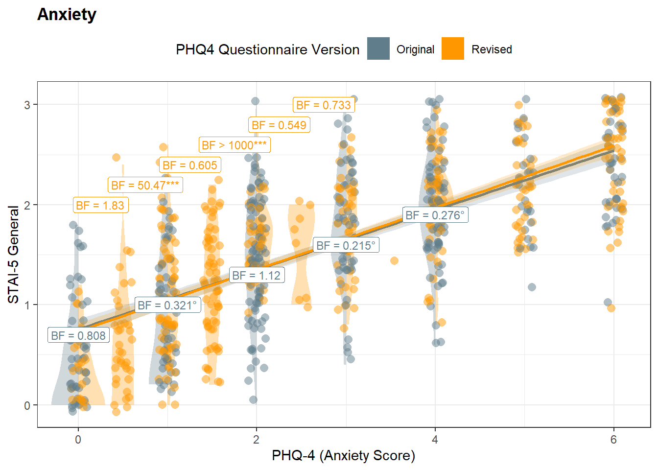

Predictive Performance

Code

m <- glm(Anxiety ~ PHQ4_Anxiety * PHQ4_Condition, data = df, family="binomial")

display(parameters::parameters(m))

Parameter	Log-Odds	SE	95% CI	z	p
(Intercept)	-3.44	0.40	(-4.28, -2.71)	-8.63	< .001
PHQ4 Anxiety	0.40	0.10	(0.22, 0.60)	4.14	< .001
PHQ4 Condition (Revised)	0.07	0.53	(-0.97, 1.14)	0.14	0.890
PHQ4 Anxiety × PHQ4 Condition (Revised)	-0.03	0.13	(-0.29, 0.23)	-0.22	0.822

Code

p_gad <- m |> 
  estimate_relation(length=20) |> 
  ggplot(aes(x=PHQ4_Anxiety, y=Predicted)) +
  geom_ribbon(aes(ymin=CI_low, ymax=CI_high, fill=PHQ4_Condition), alpha=0.2) +
  geom_line(aes(color=PHQ4_Condition), linewidth=1) +
  scale_fill_manual(values = colors) +
  scale_color_manual(values = colors) +
  scale_y_continuous(labels=scales::percent) +
  labs(y = "Probability of Anxiety",
       x= "PHQ-4 (Anxiety Score)",
       title = "Anxiety Disorder",
       fill = "Questionnaire Version",
       color = "Questionnaire Version") +
  theme_minimal()  +
  theme(plot.title = element_text(face="bold"),
        legend.position = "none")

Code

p_gadroc <- make_roc(m)

(p_gad / p_gadroc) + plot_layout(guides="collect")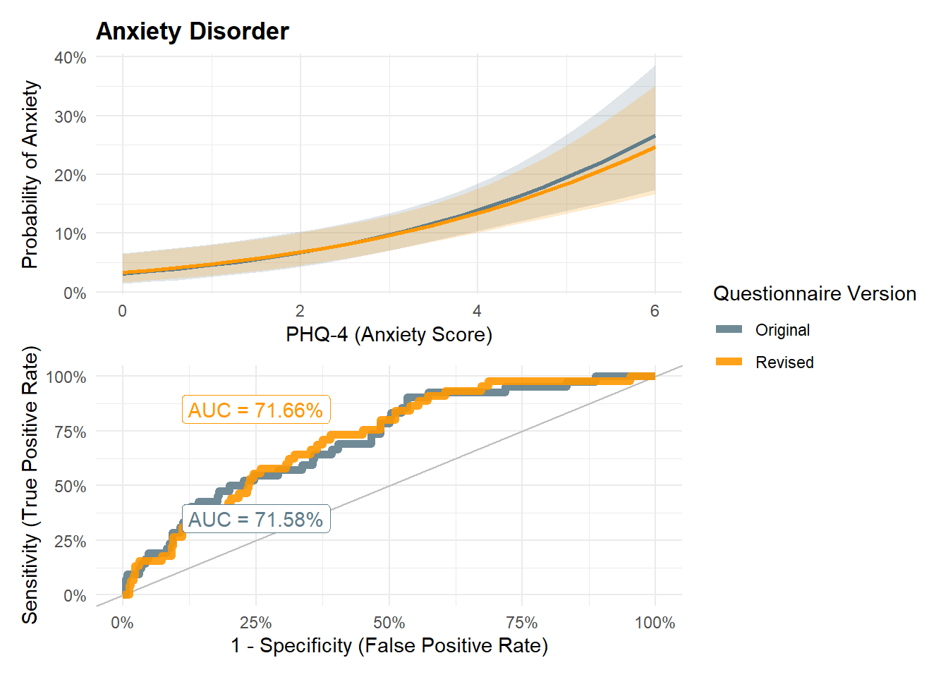

Correlation Difference

Whole Sample

Code

bootstrap_diffs <- function(df_original, df_revised) {
  dat <- data.frame()
  for(i in 1:2000) {
    newdf_ori <- df_original[sample(nrow(df_original), replace = TRUE), ]
    newdf_rev <- df_revised[sample(nrow(df_revised), replace = TRUE), ]
    
    r_depression_ori = cor.test(newdf_ori$BDI2_Total, newdf_ori$PHQ4_Depression)$estimate
    r_depression_rev = cor.test(newdf_rev$BDI2_Total, newdf_rev$PHQ4_Depression)$estimate
    r_anxiety_ori = cor.test(newdf_ori$STAI5_General, newdf_ori$PHQ4_Anxiety)$estimate
    r_anxiety_rev = cor.test(newdf_rev$STAI5_General, newdf_rev$PHQ4_Anxiety)$estimate
    
    dat <- rbind(dat,
      data.frame(
        d_r_depression = r_depression_rev - r_depression_ori,
        d_r_anxiety = r_anxiety_rev - r_anxiety_ori,
        iteration = i
      )
    )
  }
  dat
}


dat <- bootstrap_diffs(
  filter(df, PHQ4_Condition == "Original"),
  filter(df, PHQ4_Condition == "Revised"))

dat |> 
  pivot_longer(cols = c(d_r_depression, d_r_anxiety)) |>
  ggplot(aes(x = value)) +
  geom_density(aes(fill = name), alpha = 0.5) +
  geom_vline(xintercept = 0, linetype = "dashed") +
  theme_bw() +
  labs(x = "Difference in Correlation", y = "")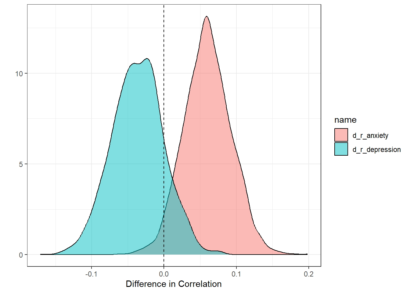

Subsamples

Code

dat <- data.frame()
for(cat in c("Minimal - Mild", "Moderate - Severe")) {
  dat <- rbind(
    dat,
    bootstrap_diffs(
      filter(df, PHQ4_Condition == "Original", BDI2_Category == cat),
      filter(df, PHQ4_Condition == "Revised", BDI2_Category == cat)) |> 
      mutate(Subsample = paste("Depression:", cat)),
    bootstrap_diffs(
      filter(df, PHQ4_Condition == "Original", STAI5_Category == cat),
      filter(df, PHQ4_Condition == "Revised", STAI5_Category == cat)) |> 
      mutate(Subsample = paste("Anxiety:", cat)) 
  )
}


dat <- dat |> 
  separate(Subsample, into = c("Type", "Subsample"), sep = ":") |>
  pivot_longer(cols = c(d_r_depression, d_r_anxiety)) |>
  filter(!(Type == "Depression" & name=="d_r_anxiety") & 
           !(Type == "Anxiety" & name=="d_r_depression")) |> 
  mutate(Type = ifelse(Type == "Depression", paste(Type, "(BDI-II)"), paste(Type, "(STAI-5)"))) |> 
  mutate(Type = fct_rev(Type)) 

p_cor <- dat |> 
  ggplot(aes(x = value)) +
  geom_density(aes(fill = name), alpha = 0.9, color="white") +
  geom_vline(xintercept = 0, linetype = "dashed") +
  geom_text(data=summarize(dat, pd = insight::format_p(bayestestR::pd_to_p(
    as.numeric(pd(value)), direction="one-sided"), stars=TRUE), 
                           .by=c("Subsample", "Type")),
            aes(label=pd, x=0.3, y=5)) +
  theme_bw() +
  labs(x = "Difference in Correlation (PHQ4 Revised - Original)", y = "") +
  facet_grid(Type~Subsample)  +
  scale_fill_manual(values = c("d_r_depression"="#3F51B5", "d_r_anxiety"="#E91E63"), guide="none") +
  theme(axis.ticks.y = element_blank(), 
        axis.text.y = element_blank(),
        strip.background = element_rect(color=NA))
p_cor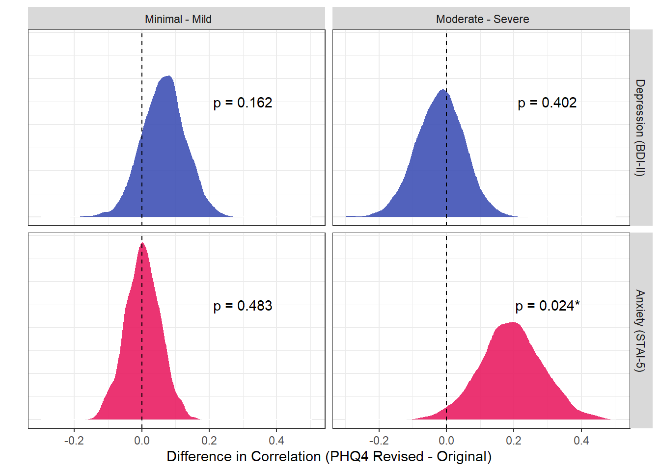

Figures

Code

p_a <- (p_dep + theme(legend.position='none')) / 
              (p_anx  + theme(legend.position='none')) +
  plot_annotation(title="A.")
            
p_b <- p_cor + plot_annotation(title="B.")

p_c <- ((p_mdd / p_mddroc) | (p_gad / p_gadroc)) + patchwork::plot_layout(guides = "collect") + patchwork::plot_annotation(title="C.", theme=theme(legend.position='left'))

(wrap_elements(p_a) | wrap_elements(p_b)) / wrap_elements(p_c)