Show figure code
df <- bayestestR::simulate_correlation(n=500, r=0.7)
df |>
  ggplot(aes(x=V1, y=V2)) +
  geom_point() +
  geom_smooth(method="lm", formula = 'y ~ x', se=FALSE, linewidth=2, color="red") +
theme_bw()@ LaPsyDé

![]()


df <- bayestestR::simulate_correlation(n=500, r=0.7)
df |>
ggplot(aes(x=V1, y=V2)) +
geom_point() +
geom_smooth(method="lm", formula = 'y ~ x', se=FALSE, linewidth=2, color="red") +
theme_bw()df |>
ggplot(aes(x=V1, y=V2)) +
geom_point() +
geom_smooth(method="lm", formula = 'y ~ x', se=FALSE, linewidth=2, color="red") +
stat_ellipse(type = "norm", color="blue", linewidth=2) +
theme_bw()ggplot(df, aes(x=V1, y=V2)) +
geom_point(alpha=0) +
geom_vline(xintercept = 0, linetype="dotted") +
geom_abline(intercept = 1, slope = 3, color="red", linewidth=2) +
geom_segment(aes(x = 0, y = 1, xend = 1, yend = 1), linewidth=1,
color="green", linetype="dashed") +
geom_segment(aes(x = 1, y = 1, xend = 1, yend = 4), linewidth=1,
color="green", linetype="solid", arrow=arrow(length = unit(0.1, "inches"))) +
geom_segment(aes(x = 0, y = 0, xend = 0, yend = 1), linewidth=1,
color="blue", linetype="solid", arrow=arrow(length = unit(0.1, "inches"))) +
geom_point(aes(x = 0, y = 0), color="purple", size=8, shape="+") +
labs(x="x", y="y") +
theme_bw() +
coord_cartesian(xlim = c(-1, 1.5), ylim = c(-3, 4))p <- mtcars |>
ggplot(aes(x=qsec, y=mpg)) +
geom_point(alpha=0.7, size=6) +
geom_smooth(method="lm", formula = 'y ~ x', se=FALSE, linewidth=2) +
geom_segment(aes(x = qsec, y = mpg, xend = qsec, yend = predict(lm(mpg ~ qsec, data=mtcars))),
color="red", linetype="dotted", linewidth=1) +
theme_bw() +
labs(x="x", y="y", title="The residuals are the vertical distances between each point and the line.")
p2 <- data.frame(Error=insight::get_residuals(lm(mpg ~ qsec, data=mtcars))) |>
ggplot(aes(x=Error)) +
geom_histogram(bins=10, fill="grey", color="black") +
geom_vline(xintercept = 0, linetype="dashed") +
geom_density(data=data.frame(Error=bayestestR::distribution_normal(n=100, sd = 2)),
aes(y=after_stat(density)*40), color="#F44336", linewidth=1, adjust=1) +
geom_density(data=data.frame(Error=bayestestR::distribution_normal(n=100, sd = 3)),
aes(y=after_stat(density)*50), color="#FF5722", linewidth=1, adjust=1) +
geom_density(data=data.frame(Error=bayestestR::distribution_normal(n=100, sd = 4)),
aes(y=after_stat(density)*60), color="#FF9800", linewidth=1, adjust=1) +
geom_point(aes(y=0), size=10, shape=16, alpha=0.3) +
theme_bw() +
coord_flip() +
labs(y = "Density")
p + theme(plot.title = element_blank()) | p2model <- lm(mpg ~ qsec, data=mtcars)
p <- mtcars |>
ggplot(aes(x=qsec, y=mpg)) +
geom_smooth(method="lm", formula = 'y ~ x', se=FALSE, linewidth=2) +
theme_bw()
# Function to add normal distribution curves
add_normals <- function(p, model) {
sigma <- summary(model)$sigma # Standard deviation of residuals
n <- 100 # Number of points for each curve
for(i in 1:nrow(mtcars)) {
x_val <- mtcars$qsec[i]
y_pred <- predict(model, newdata = data.frame(qsec = x_val))
# Create a sequence of y values for the normal curve
y_seq <- seq(y_pred - 3*sigma, y_pred + 3*sigma, length.out = n)
density <- dnorm(y_seq, mean = y_pred, sd = sigma)
# Adjust density to match the scale of the plot
max_width <- 1 # Max width of areas
density_scaled <- (density / max(density)) * max_width
# Create a dataframe for each path
path_df <- data.frame(x = x_val + density_scaled, y = y_seq)
path_dfv <- data.frame(x=path_df$x[1], ymin=min(path_df$y), ymax=max(path_df$y))
# Add the path to the plot
p <- p +
geom_segment(data = path_dfv, aes(x = x, xend=x, y = ymin, yend=ymax),
color = "#FF9800", linewidth = 0.7, alpha=0.8, linetype="dotted") +
geom_path(data = path_df, aes(x = x, y = y),
color = "#FF9800", linewidth = 1, alpha=0.8)
}
p
}
# Create the final plot
p <- add_normals(p, model) +
geom_segment(aes(x = qsec, y = mpg, xend = qsec, yend = predict(lm(mpg ~ qsec, data=mtcars))),
color="red", linetype="solid", linewidth=1) +
geom_point(alpha=0.8, size=6)
p# Plot t-distribution
x <- seq(-5, 5, length.out = 1000)
y <- dt(x, df=30)
df <- data.frame(x = x, y = y)
t_value <- 2.790
df$Probability <- ifelse(df$x < -t_value, "< -t", "Smaller")
df$Probability <- ifelse(df$x > t_value, "> +t", df$Probability)
df |>
ggplot(aes(x = x, y = y)) +
geom_line() +
geom_area(aes(x = x, y = y, fill = Probability), alpha = 0.5) +
geom_segment(data=data.frame(x=t_value, y=0),
aes(xend = t_value, yend = dt(t_value, df=30)),
color="red", linetype="solid", linewidth=1) +
geom_point(data=data.frame(x=t_value, y=dt(t_value, df=30)), color="red", size=3) +
theme_minimal() +
scale_fill_manual(values = c("red", "red", "grey")) +
labs(x = "\nt-values - standardized coefficient under the null hypothesis", y = "Probability",
title = paste0("t-Distribution (df=30); ", "t-value = ", round(t_value, 2), "\n"))model <- lm(mpg ~ qsec, data=mtcars) # Fit linear regression
true_coef <- coef(model)[2] # Extract slope coefficient
coefs <- c() # Initialize an empty vector of coefs
for (i in 1:5000) { # Repeat the process 500 times
new_sample <- mtcars[sample(1:nrow(mtcars), replace = TRUE), ] # Sample new data
new_model <- lm(mpg ~ qsec, data=new_sample) # recompute the model
coefs <- c(coefs, coef(new_model)[2]) # Append the coef to the vector
}data.frame(coefs = coefs) |>
ggplot(aes(x = coefs)) +
geom_density(fill="orange") +
geom_vline(xintercept = true_coef, color="red", linetype="dashed", linewidth=2) +
theme_minimal() +
labs(x = "Coefficient", y = "Frequency",
title = "Distribution of coefficients from 5000 bootstrapped samples\n") +
coord_cartesian(xlim = c(-0.5, NA))

bayestestR exists to convert between the two indices.
bayestestR::p_to_pd(c(0.05, 0.01, 0.001), direction = "two-sided")[1] 0.9750 0.9950 0.9995bayestestR::pd_to_p(c(0.90, 0.95), direction = "two-sided")[1] 0.2 0.1
data.frame(Coefficient = coefs) |>
  ggplot(aes(x=Coefficient)) +
  geom_density(fill="blue") +
  geom_area(data=data.frame(x=c(-0.42, 0.42)), aes(x=x, y=2), fill="red", alpha=0.5) +
  coord_cartesian(xlim=c(-0.6, 3.5))
bayestestR::rope(coefs, range = c(-0.42, 0.42), ci = 1.00)# Proportion of samples inside the ROPE [-0.42, 0.42]:
inside ROPE
-----------
0.66 % # ci=0.95 is the default setting for rope()
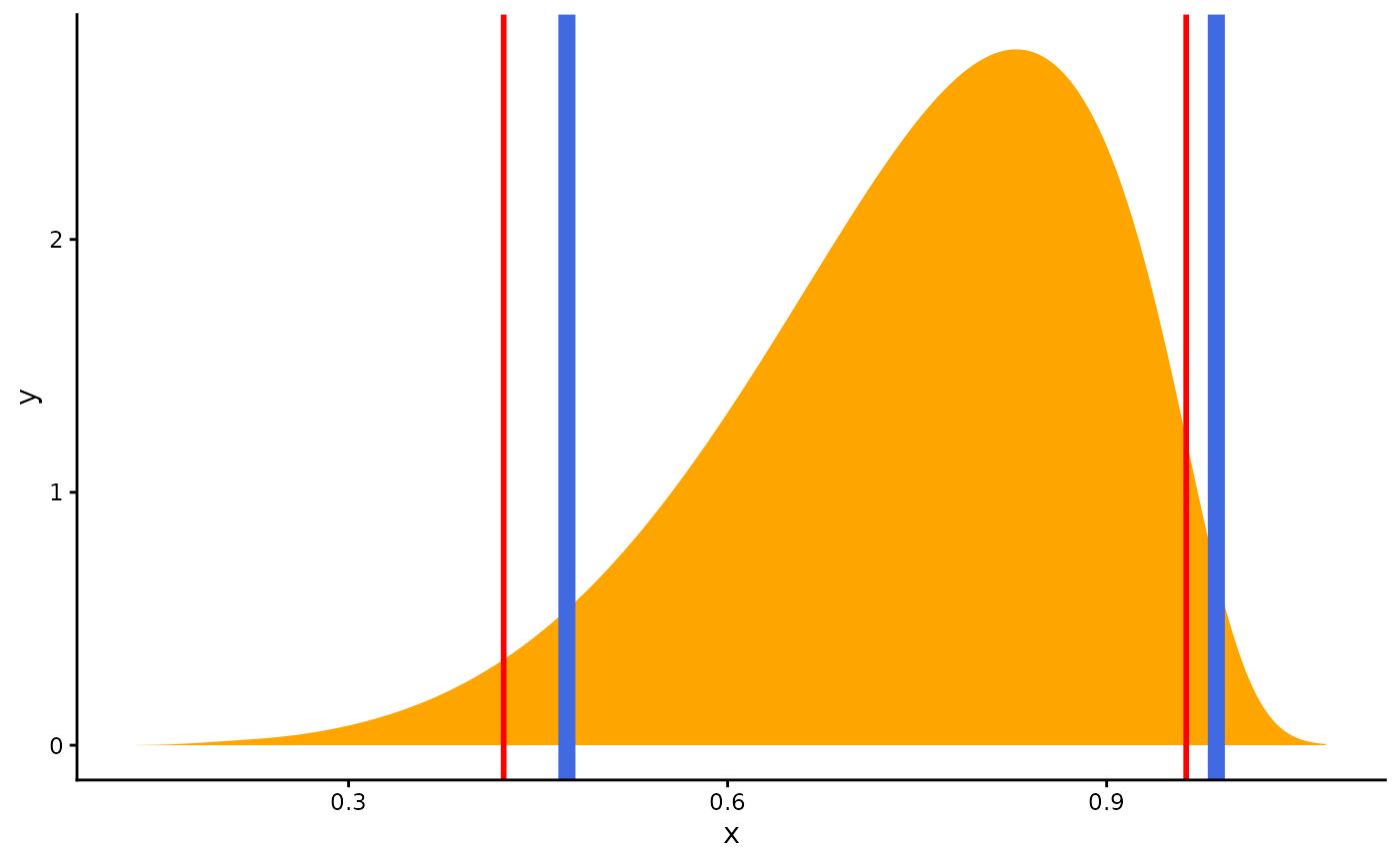
result <- bayestestR::rope(coefs, range = c(-0.42, 0.42), ci = 0.95)
result# Proportion of samples inside the ROPE [-0.42, 0.42]:
inside ROPE
-----------
0.00 % # The results can be plotted
plot(result)

Thank you!
![]()