Ex-Gaussian models in R: A Tutorial

Setup

If you haven’t, install the easyRT package by running:

remotes::install_github("DominiqueMakowski/easyRT")

Load the necessary packages.

library(tidyverse)
library(easystats)
library(rtdists)
library(easyRT)

Theory

Rather than relying on default model families, such as Gaussian models, one can select models that accurately represents the distribution of their outcome variable. For instance, models based on Exponentially modified Gaussian (ex-Gaussian) distributions, which are suited to their typical skewed shape (Balota and Yap 2011; Matzke and Wagenmakers 2009).

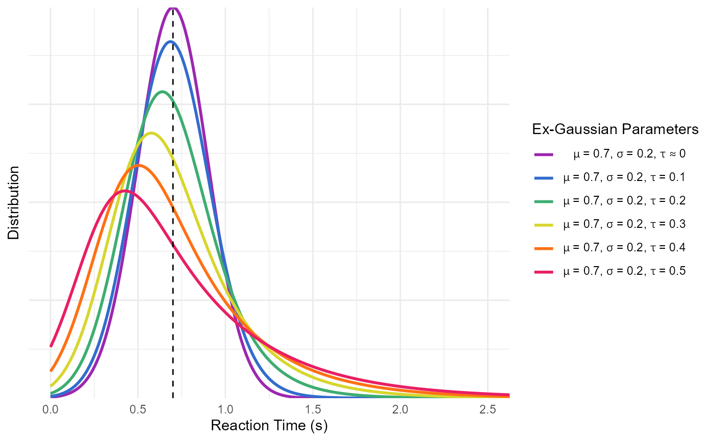
This distribution is a convolution of normal and exponential distributions and has three parameters, namely \(\mu\) (mu) and \(\sigma\) (sigma) - the mean and standard deviation of the Gaussian distribution - and \(\tau\) (tau) - the exponential component of the distribution. Intuitively, these arguments reflect the centrality, the width and the tail dominance, respectively (see figure below).

Beyond the descriptive value of these types of models, some have tried to interpret their parameters in terms of cognitive mechanisms, arguing for instance that changes in the Gaussian components reflect changes in attentional processes (e.g., “the time required for organization and execution of the motor response”; Hohle, 1965), whereas changes in the exponential component reflect changes in intentional (i.e., decision-related) processes (Kieffaber et al. 2006). However, Matzke and Wagenmakers (2009) demonstrate that there is no direct correspondence between ex-Gaussian parameters and cognitive mechanisms, and underline their value primarily as descriptive tools, rather than models of cognition per se.

Descriptively, the three parameters can be interpreted as:

• Mu \(\mu\): The location / centrality of the RTs. Would correspond to the mean in a symmetrical distribution.
• Sigma \(\sigma\): The variability and dispersion of the RTs. Akin to the standard deviation in normal distributions.
• Tau \(\tau\): Tail weight / skewness of the distribution.

Note that these parameters are not independent with respect to distribution characteristics: below is an example of different distributions with the same location and dispersion. Although only the tail weight parameter is changed, the whole dsitribution appears to shift is centre of mass. Hence, one should be careful note to interpret the values of mu directly as the “mean” or the distribution “peak” and sigma as the SD or the “width”.

Example of Ex-gaussian Distributions with same location and dispersion.

Balota, David A, and Melvin J Yap. 2011. “Moving Beyond the Mean in Studies of Mental Chronometry: The Power of Response Time Distributional Analyses.” Current Directions in Psychological Science 20 (3): 160–66.

Kieffaber, Paul D, Emily S Kappenman, Misty Bodkins, Anantha Shekhar, Brian F O’Donnell, and William P Hetrick. 2006. “Switch and Maintenance of Task Set in Schizophrenia.” Schizophrenia Research 84 (2-3): 345–58.

Matzke, Dora, and Eric-Jan Wagenmakers. 2009. “Psychological Interpretation of the Ex-Gaussian and Shifted Wald Parameters: A Diffusion Model Analysis.” Psychonomic Bulletin & Review 16 (5): 798–817.