
The Beta-Gate model represents subjective ratings as a mixture of a continuous Beta distribution with additional point masses at the extremes (0 and 1). This structure effectively captures common patterns in subjective rating data where respondents often select extreme values at higher rates than would be expected from a Beta distribution alone.
The Beta-Gate model corresponds to a reparametrized ordered beta model (Kubinec, 2023, doi:10.1017/pan.2022.20 ). In the ordered Beta model, the extreme values (0 and 1) arise from censoring an underlying latent process based on cutpoints ("gates"). Values falling past the gates are considered extremes (zeros and ones). The difference from the Ordered Beta is the way the cutpoints are defined, as well as the scale of the precision parameter phi.
It differs from the Zero-One-Inflated Beta (ZOIB) model in that the ZOIB model has zoi
and coi parameters, directly controlling the likelihood of extreme values. Instead,
Beta-Gate uses pex and bex to define "cutpoints" after which extreme values become likely.
In an ordered beta framework, the boundary probabilities arise through a single underlying
ordering process (the location of the cutpoints on the latent scale). In a ZOIB framework,
the boundaries are more like additional mass points inserted into a beta distribution.
In Beta-gate models, extreme values arise naturally from thresholding a single latent process.
Usage
rcogmod_betagate(n, mu = 0.5, phi = 3, pex = 0.1, bex = 0.5)

dcogmod_betagate(x, mu = 0.5, phi = 3, pex = 0.1, bex = 0.5, log = FALSE)

cogmod_betagate_lpdf_expose()

cogmod_betagate_stanvars()

cogmod_betagate(
  link_mu = "logit",
  link_phi = "softplus",
  link_pex = "logit",
  link_bex = "logit"
)

log_lik_cogmod_betagate(i, prep)

posterior_predict_cogmod_betagate(i, prep, ...)

posterior_epred_cogmod_betagate(prep)
Arguments
- n
Number of simulated values.
- mu
Mean of the underlying Beta distribution (
0 < mu < 1).- phi
Precision parameter of the underlying Beta distribution (must be strictly positive). Can be conceptualized as an "agreement" indicator: higher
phimeans less dispersion (more agreement) among ratings, holdingmufixed. Note: In many implementations,phiis parametrized differently, and correspond to the double of ourphiargument (cogmod'sphi= standard'sphi* 2). Our parametrization Makes itphi = 1corresponds to uniform whenmu = 0.5, which makes setting priors more convenient (e.g., on the logit scale)- pex
Controls the location of the lower and upper boundary gates (
0 <= pex <= 1). It defines the total probability mass allocated to the extremes (0 or 1). Higherpexincreases the probability of extreme values (0 or 1).- bex
Balances the extreme probability mass
pexbetween 0 and 1 (0 <= bex <= 1). A balance of0.5means that the 'gates' are symmetrically placed around the center of the distribution, and values higher or lower than0.5will shift the relative "ease" of crossing the gates towards 1 or 0, respectively.- x
Vector of quantiles (values at which to evaluate the density). Must be between 0 and 1, inclusive.
- log
Logical; if TRUE, returns the log-density.
- link_mu, link_phi, link_pex, link_bex
Link functions for the parameters.
- i, prep
For brms' functions to run: index of the observation and a
brmspreparation object.- ...
Additional arguments.
Value
rcogmod_betagate() returns a numeric vector of n simulated
ratings on the unit interval [0, 1], including the exact 0s and 1s
produced by the gates. dcogmod_betagate() returns the density at each
element of x - the log density if log = TRUE - recycled to the length
of the longest argument; at 0 and 1 it is the probability mass rather
than a density. cogmod_betagate() returns a brms::custom_family
object, to put on a brms::bf() formula. cogmod_betagate_stanvars()
returns a brms::stanvars object holding the family's Stan functions
block, to pass to brms::brm(), and cogmod_betagate_lpdf_expose()
compiles that Stan code and returns it as an R function, for checking the
density outside of a model. The remaining functions are brms
post-processing methods, called by brms rather than directly:
log_lik_cogmod_betagate() returns a numeric vector holding one
log-likelihood value per posterior draw for observation i,
posterior_predict_cogmod_betagate() a draws x 1 matrix of ratings
simulated for observation i, and posterior_epred_cogmod_betagate() a
draws x observations matrix of expected ratings.
Details
Special cases:
When
pex = 0: Pure Beta distribution with meanmuand precisionphi * 2.When
pex = 1: Pure Bernoulli distribution withP(1) = bex,P(0) = 1-bex.When
bex = 0andpex = 1: All mass at 0.When
bex = 1andpex = 1: All mass at 1.
Psychological Interpretation:
mu: Can be interpreted as the underlying average tendency or preference strength, disregarding extreme "all-or-nothing" responses.phi: Reflects the certainty or consistency of the non-extreme responses. Higherphiindicates responses tightly clustered aroundmu(more certainty), while lowerphi(especiallyphi = 1) suggests more uniform or uncertain responses.pex: Represents the overall tendency towards extreme responding (choosing 0 or 1). This could reflect individual response styles (e.g., acquiescence, yea-saying/nay-saying) or properties of the item itself (e.g., polarizing questions).bex: Indicates the direction of the extreme response bias.bex > 0.5suggests a bias for producing ones more easily, whilebex < 0.5suggests a bias towards zero.
References
Kubinec, R. (2023). Ordered beta regression: a parsimonious, well-fitting model for continuous data with lower and upper bounds. Political Analysis, 31(4), 519-536.
Examples
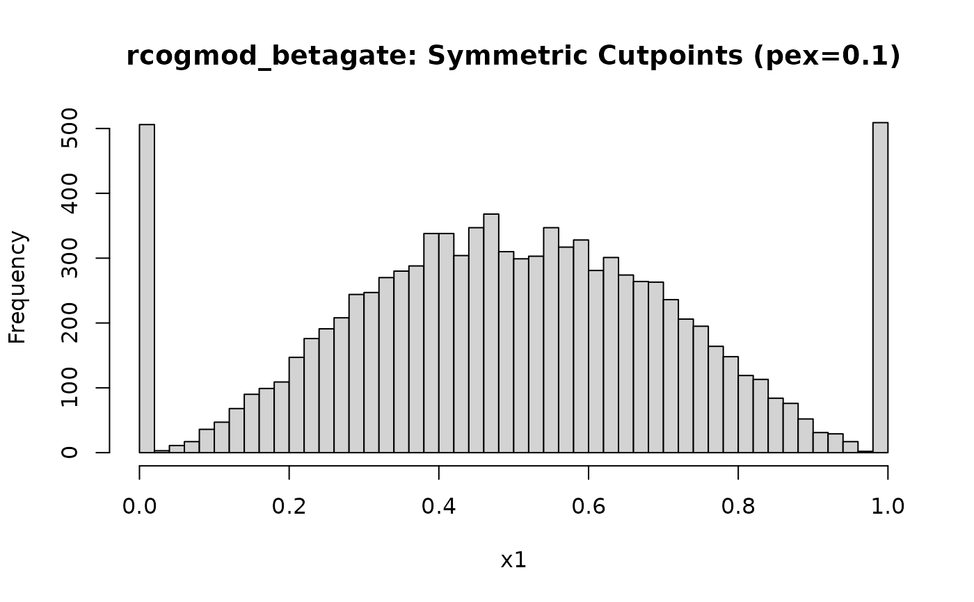
# Symmetric gates (c0=0.05, c1=0.95), pex=0.1, bex=0.5
x1 <- rcogmod_betagate(10000, mu = 0.5, phi = 3, pex = 0.1, bex = 0.5)
hist(x1, breaks=50, main="rcogmod_betagate: Symmetric Cutpoints (pex=0.1)")
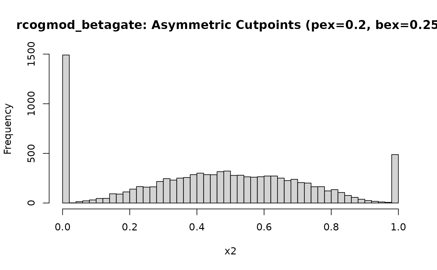
 # Asymmetric gates (c0=0.15, c1=0.95), pex=0.2, bex=0.25
x2 <- rcogmod_betagate(10000, mu = 0.5, phi = 3, pex = 0.2, bex = 0.25)
hist(x2, breaks=50, main="rcogmod_betagate: Asymmetric Cutpoints (pex=0.2, bex=0.25)")
# Asymmetric gates (c0=0.15, c1=0.95), pex=0.2, bex=0.25
x2 <- rcogmod_betagate(10000, mu = 0.5, phi = 3, pex = 0.2, bex = 0.25)
hist(x2, breaks=50, main="rcogmod_betagate: Asymmetric Cutpoints (pex=0.2, bex=0.25)")
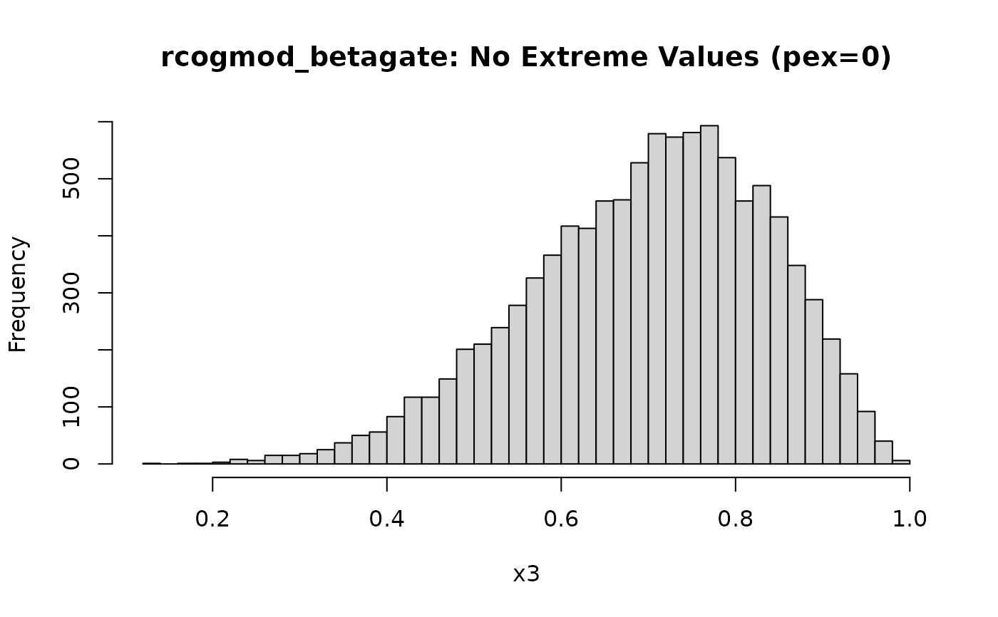
 # No gating (pure Beta)
x3 <- rcogmod_betagate(10000, mu = 0.7, phi = 5, pex = 0, bex = 0.5)
hist(x3, breaks=50, main="rcogmod_betagate: No Extreme Values (pex=0)")
# No gating (pure Beta)
x3 <- rcogmod_betagate(10000, mu = 0.7, phi = 5, pex = 0, bex = 0.5)
hist(x3, breaks=50, main="rcogmod_betagate: No Extreme Values (pex=0)")
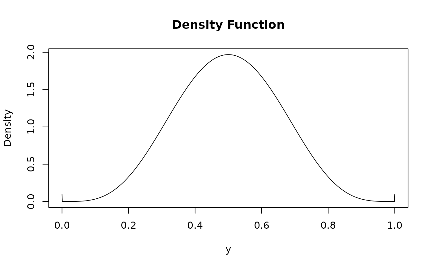
 x <- seq(0, 1, length.out = 1001)
densities <- dcogmod_betagate(x, mu = 0.5, phi = 5, pex = 0.2, bex = 0.5)
plot(x, densities, type = "l", main = "Density Function", xlab = "y", ylab = "Density")
x <- seq(0, 1, length.out = 1001)
densities <- dcogmod_betagate(x, mu = 0.5, phi = 5, pex = 0.2, bex = 0.5)
plot(x, densities, type = "l", main = "Density Function", xlab = "y", ylab = "Density")
 if (FALSE) { # \dontrun{
# Needs cmdstanr and a CmdStan toolchain, which live outside CRAN - see the
# package website to install them. Not run under R CMD check, which executes
# every example in one R session: once brms has fitted a model there (the
# cogmod_inits() and p_outlier() examples do), rstan is live in the process
# and loading an exposed Stan function next to it segfaults on Linux.
lpdf <- cogmod_betagate_lpdf_expose()
lpdf(y = 0.5, mu = 0.6, phi = 10, pex = 0.2, bex = 0.5)
} # }
if (FALSE) { # \dontrun{
# Needs cmdstanr and a CmdStan toolchain, which live outside CRAN - see the
# package website to install them. Not run under R CMD check, which executes
# every example in one R session: once brms has fitted a model there (the
# cogmod_inits() and p_outlier() examples do), rstan is live in the process
# and loading an exposed Stan function next to it segfaults on Linux.
lpdf <- cogmod_betagate_lpdf_expose()
lpdf(y = 0.5, mu = 0.6, phi = 10, pex = 0.2, bex = 0.5)
} # }