Simulate Data
df <- data.frame()
for(x in seq(0.1, 0.9, by = 0.1)) {
  score <- rchoco(n = 100, p = 0.4 + x / 2, confright = 0.4 + x / 3,
                  confleft = 1-x, pex = 0.03, bex = 0.6, pmid = 0)
  df <- rbind(df, data.frame(x = x, score = score))
}

df |>
  ggplot(aes(x = score, y = after_stat(density))) +
  geom_histogram(bins = 100, fill = "#2196F3") +
  labs(title = "Rating Distribution", x = "Score", y = "Density") +
  theme_minimal()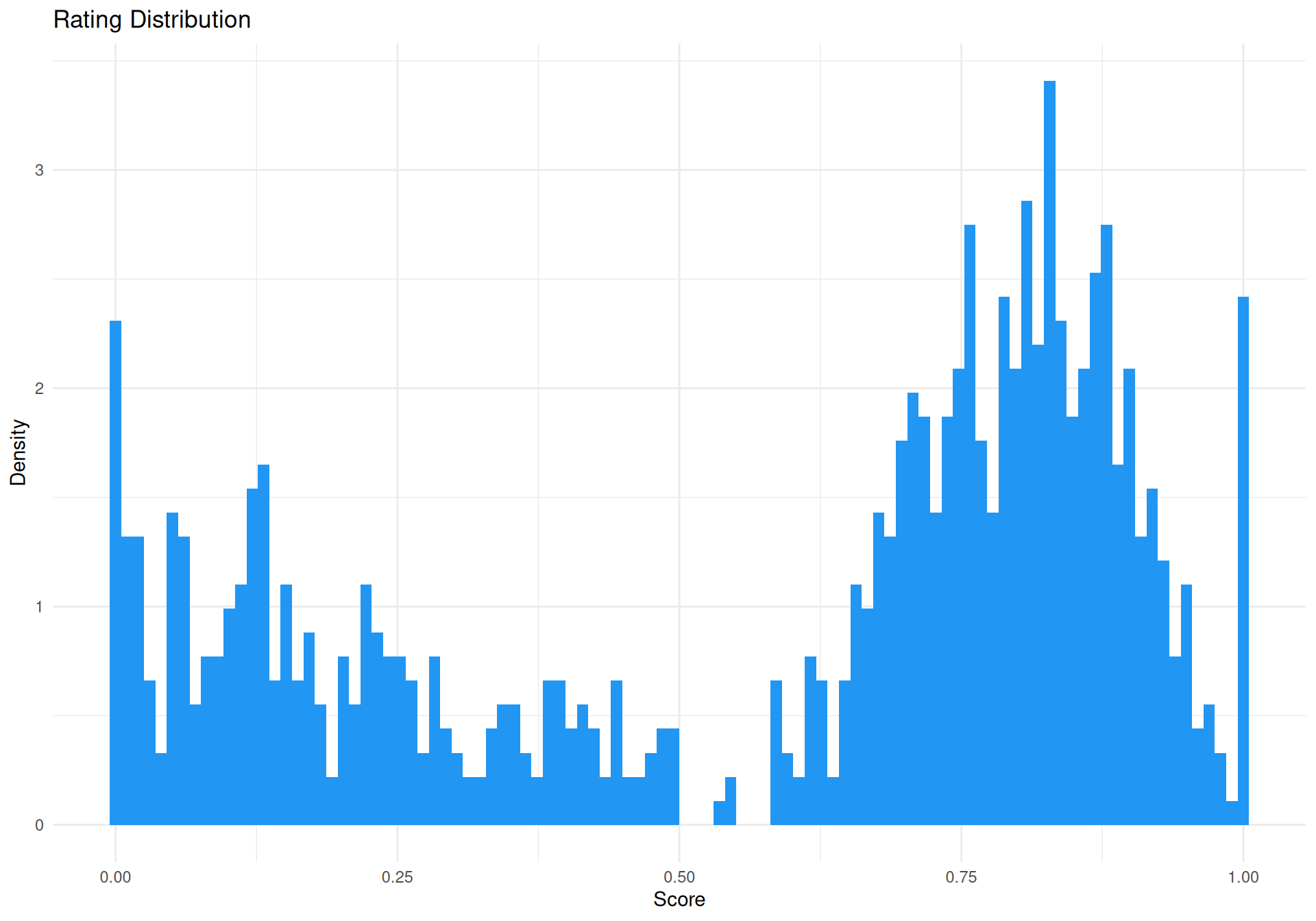
Models
ZOIB Model
The Zero-One Inflated Beta (ZOIB) model assumes that the data can be modeled as a mixture of two logistic regression processes for the boundary values (0 and 1) and a beta regression process for the continuous proportions in-between.
f <- bf(
  score ~ x,
  phi ~ x,
  zoi ~ x,
  coi ~ x,
  family = zero_one_inflated_beta()
)

m_zoib <- brm(f,
  data = df, family = zero_one_inflated_beta(), init = 0,
  chains = 4, iter = 500, backend = "cmdstanr"
)

m_zoib <- brms::add_criterion(m_zoib, "loo")  # For later model comparison

saveRDS(m_zoib, file = "models/m_zoib.rds")
XBX Model
Kosmidis & Zeileis (2024) introduce a generalization of the classic beta regression model with extended support [0, 1]. Specifically, the extended-support beta distribution (xbeta) leverages an underlying symmetric four-parameter beta distribution with exceedence parameter nu to obtain support [-nu, 1 + nu] that is subsequently censored to [0, 1] in order to obtain point masses at the boundary values 0 and 1.
f <- bf(
  score ~ x,
  phi ~ x,
  kappa ~ x,
  family = xbeta()
)

m_xbx <- brm(f,
  data = df, family = xbeta(), init = 0,
  chains = 4, iter = 500, backend = "cmdstanr"
)

m_xbx <- brms::add_criterion(m_xbx, "loo")  # For later model comparison

saveRDS(m_xbx, file = "models/m_xbx.rds")
Beta-Gate Model
The Beta-Gate model corresponds to a reparametrized Ordered Beta model (Kubinec, 2023). In this model, observed 0s and 1s represent instances where the underlying continuous response tendency fell beyond lower or upper boundary points (‘gates’).
f <- bf(
  score ~ x,
  phi ~ x,
  pex ~ x,
  bex ~ x,
  family = betagate()
)

m_betagate <- brm(f,
  data = df, family = betagate(), stanvars = betagate_stanvars(), init = 0,
  chains = 4, iter = 500, backend = "cmdstanr"
)

m_betagate <- brms::add_criterion(m_betagate, "loo")  # For later model comparison

saveRDS(m_betagate, file = "models/m_betagate.rds")
CHOCO Model
See the documentation of the Choice-Confidence (CHOCO).
f <- bf(
  score ~ x,
  confright ~ x,
  confleft ~ x,
  precright ~ x,
  precleft ~ x,
  pex ~ x,
  bex ~ x,
  pmid = 0,
  family = choco()
)

m_choco <- brm(f,
  data = df, family = choco(), stanvars = choco_stanvars(), init = 0,
  chains = 4, iter = 500, backend = "cmdstanr"
)

m_choco <- brms::add_criterion(m_choco, "loo")  # For later model comparison

saveRDS(m_choco, file = "models/m_choco.rds")
Model Comparison
#> Loading required namespace: rstanModel Fit
We can compare these models together using the loo package, which shows that CHOCO provides a significantly better fit than the other models.
Code
# loo::loo_compare(m_zoib, m_xbx, m_betagate, m_choco) |>
#   parameters(include_ENP = TRUE)
Sampling Duration
rbind(
  data_modify(attributes(m_zoib$fit)$metadata$time$chain, Model="ZOIB"),
  data_modify(attributes(m_xbx$fit)$metadata$time$chain, Model="XBX"),
  data_modify(attributes(m_betagate$fit)$metadata$time$chain, Model="Beta-Gate"),
  data_modify(attributes(m_choco$fit)$metadata$time$chain, Model="CHOCO")
) |>
  ggplot(aes(x = Model, y = total, fill = Model)) +
  geom_boxplot() +
  labs(y = "Sampling Duration (s)") +
  scale_fill_material_d(guide = "none") +
  scale_y_log10() +
theme_minimal() 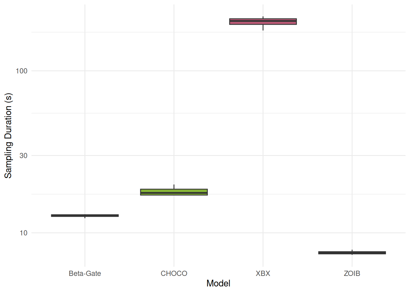
Posterior Predictive Check
Running posterior predictive checks allows to visualize the predicted distributions from various models. We can see how typical Beta-related models fail to capture the bimodal nature of the data, which is well captured by the CHOCO model.
Note: iterations controls the actual number of iterations used (e.g., for the point-estimate) and keep_iterations the number included.
Code
pred <- rbind(
  estimate_prediction(m_zoib, keep_iterations = 50, iterations = 50) |>
    reshape_iterations() |>
    data_modify(Model = "ZOIB"),
  estimate_prediction(m_xbx, keep_iterations = 50, iterations = 50) |>
    reshape_iterations() |>
    data_modify(Model = "XBX"),
  estimate_prediction(m_betagate, keep_iterations = 50, iterations = 50) |>
    reshape_iterations() |>
    data_modify(Model = "Beta-Gate"),
  estimate_prediction(m_choco, keep_iterations = 50, iterations = 50) |>
    reshape_iterations() |>
    data_modify(Model = "CHOCO")
)

df |>
  ggplot(aes(x = score, y = after_stat(density))) +
  geom_histogram(bins = 100, fill = "#2196F3") +
  labs(title = "Rating Distribution", x = "Score", y = "Density") +
  theme_minimal() +
  geom_histogram(
    data = pred, aes(x = iter_value, group = as.factor(iter_group)),
    bins = 100, alpha = 0.02, position = "identity", fill = "#FF5722"
  ) +
  facet_wrap(~Model)
Effect Visualisation
We can see how the predicted distribution changes as a function of x and gets “pushed” to the right. Moreover, we can also visualize the effect of x on specific parameters, showing that it mostly affects the parameter conf (the mean confidence - i.e., central tendency - on the right side), confleft (the relative confidence of the left side), and mu, which corresponds to the p probability of answering on the right. This is consistent with our expectations, and reflects the larger and more concentrated mass on the right of the scale for higher value of x (in brown).
Code
p1 <- estimate_prediction(m_choco, data = "grid", length = 4, keep_iterations = 500, iterations = 500) |>
  reshape_iterations() |>
  ggplot(aes(x = iter_value, fill = as.factor(x))) +
  geom_histogram(alpha = 0.6, bins = 100, position = "identity") +
  scale_fill_bluebrown_d() +
  labs(x = "Rating") +
  theme_minimal()
p1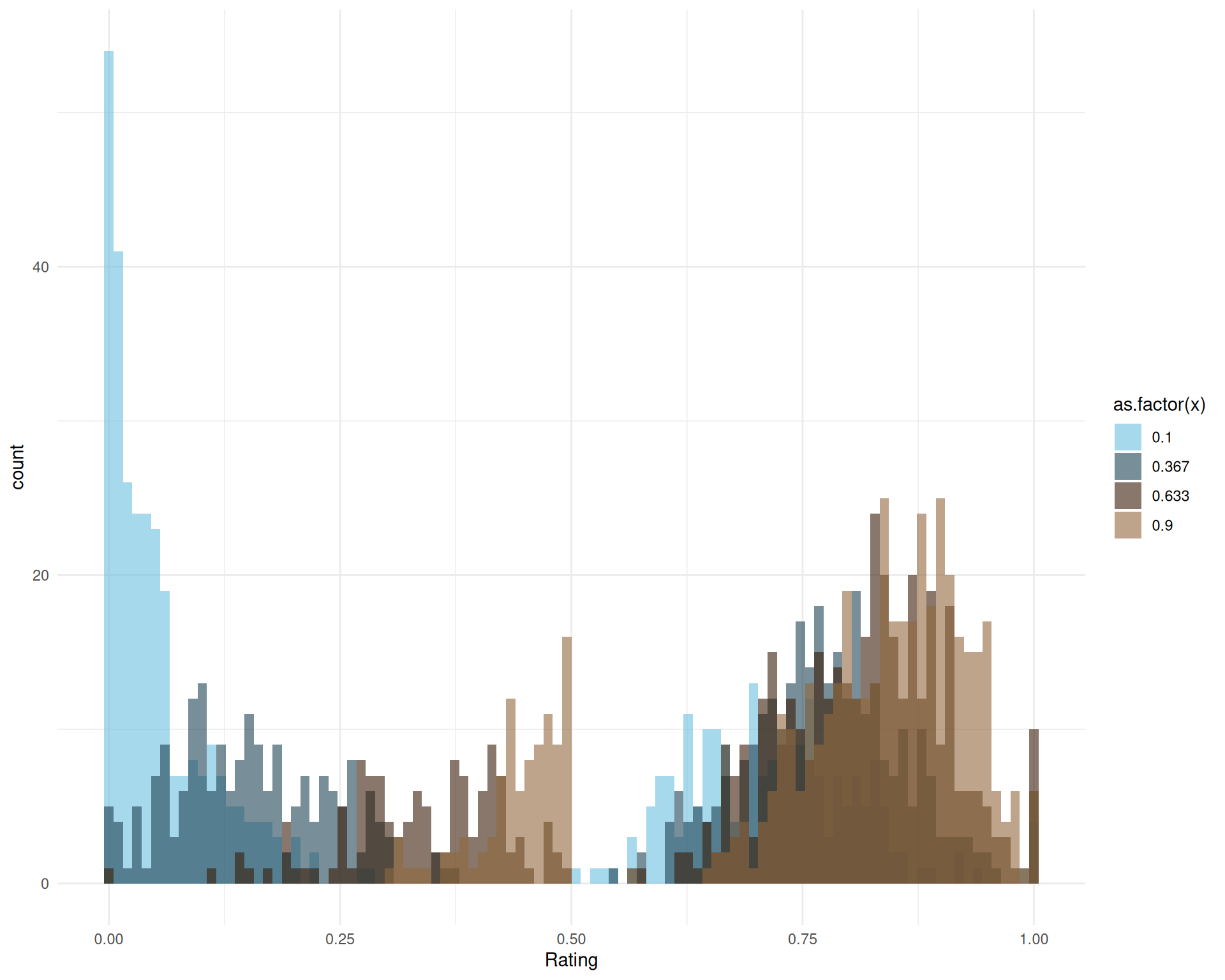
Code
# # Predict various parameters
# pred_params <- data.frame()
# for(param in c("mu", "confright", "confleft", "precright", "precleft", "pex")) {
#   pred_params <- m_choco |>
#     estimate_prediction(data = "grid", length = 20, predict = param) |>
#     as.data.frame() |>
#     data_modify(Parameter = param) |>
#     rbind(pred_params)
# }
#
# p2 <- pred_params |>
#   ggplot(aes(x = x, y = Predicted)) +
#   geom_ribbon(aes(ymin = CI_low, ymax = CI_high, fill = Parameter), alpha = 0.2) +
#   geom_line(aes(color = Parameter), linewidth = 1) +
#   facet_wrap(~Parameter, scales = "free_y", ncol=3) +
#   scale_fill_viridis_d() +
#   scale_color_viridis_d() +
#   theme_minimal()
# p2