# using Downloads, CSV, DataFrames, Random
# using Turing, Distributions
# using GLMakie
# using LinearAlgebra
# # Define the monotonic function
# function monotonic(scale::Vector{Float64}, i::Int)
# if i == 0
# return 0.0
# else
# return length(scale) * sum(scale[1:i])
# end
# end
# # Test
# using RDatasets
# data = dataset("datasets", "mtcars")
# # Response variable
# y = data[!, :MPG]
# x = data[!, :Gear]
# # Number of observations
# N = length(y)
# # Length of simplex
# Jmo = maximum(x)
# # Prior concentration for the simplex (using a uniform prior for simplicity)
# con_simo_1 = ones(Jmo)
# # Turing Model Specification
# @model function monotonic_model(y, x, N, Jmo, con_simo_1)
# # Parameters
# Intercept ~ Normal(19.2, 5.4)
# simo_1 ~ Dirichlet(con_simo_1)
# sigma ~ truncated(Normal(0, 5.4), 0, Inf)
# bsp ~ Normal(0, 1)
# # Linear predictor
# mu = Vector{Float64}(undef, N)
# for n in 1:N
# mu[n] = Intercept + bsp * monotonic(simo_1, x[n])
# end
# # Likelihood
# y ~ MvNormal(mu, sigma)
# end
# # Run the model
# model = monotonic_model(y, x, N, Jmo, con_simo_1)
# chain = sample(model, NUTS(), 1000)
# # Display the results
# display(chain)2 Predictors
![]()
2.1 Categorical predictors (Condition, Group, …)
![]()
In the previous chapter, we have mainly focused on the relationship between a response variable and a single continuous predictor.
- Contrasts, …
2.2 Interactions
![]()
Todo.
- Nested interactions (difference between R’s formula
fac1 * fac2andfac1 / fac2and how to specify that in Julia/Turing) - Use of the
@formulamacro to create the design matrix.
2.3 Ordered predictors (Likert Scales)
Likert scales, i.e., ordered multiple discrete choices are often used in surveys and questionnaires. While such data is often treated as a continuous variable, such assumption is not necessarily valid. Indeed, distance between the choices is not necessarily equal. For example, the difference between “strongly agree” and “agree” might not be the same as between “agree” and “neutral”. Even when using integers like 1, 2, 3, 4; people might implicitly process “4” as more extreme relative to “3” as “3” to “2”.
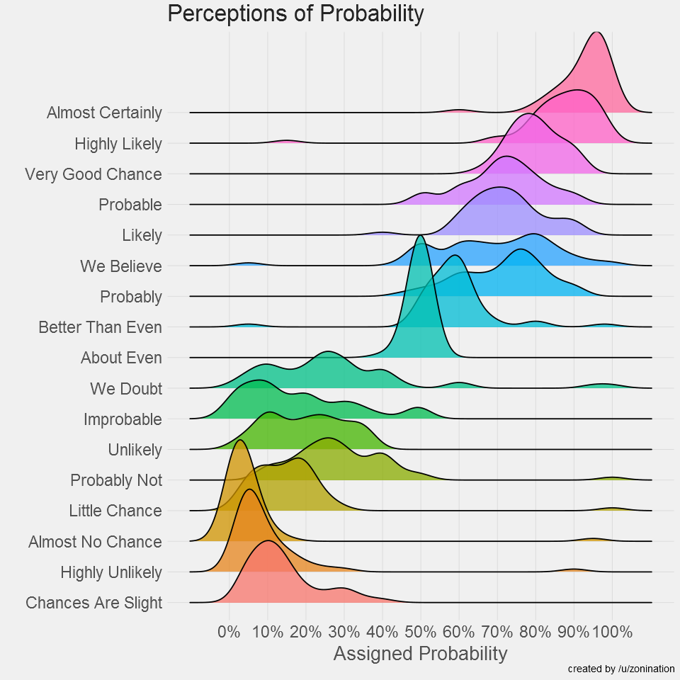
The probabilities assigned to discrete probability descriptors are not necessarily equidistant (https://github.com/zonination/perceptions)
2.3.1 Monotonic Effects
What can we do to better reflect the cognitive process underlying a Likert scale responses? Monotonic effects.
- How to do Monotonic effects in Turing?
library(brms)

m <- brm(mpg ~ mo(gear), data = mtcars, refresh=0)

# stancode(m)
m
Family: gaussian
Links: mu = identity; sigma = identity
Formula: mpg ~ mo(gear)
Data: mtcars (Number of observations: 32)
Draws: 4 chains, each with iter = 2000; warmup = 1000; thin = 1;
total post-warmup draws = 4000
Regression Coefficients:
Estimate Est.Error l-95% CI u-95% CI Rhat Bulk_ESS Tail_ESS
Intercept 16.51 1.31 14.01 19.19 1.00 2106 2213
mogear 3.88 1.02 1.81 5.86 1.00 2160 2315
Monotonic Simplex Parameters:
Estimate Est.Error l-95% CI u-95% CI Rhat Bulk_ESS Tail_ESS
mogear1[1] 0.84 0.13 0.52 0.99 1.00 2698 1862
mogear1[2] 0.16 0.13 0.01 0.48 1.00 2698 1862
Further Distributional Parameters:
Estimate Est.Error l-95% CI u-95% CI Rhat Bulk_ESS Tail_ESS
sigma 5.02 0.68 3.90 6.58 1.00 2850 2485
Draws were sampled using sampling(NUTS). For each parameter, Bulk_ESS
and Tail_ESS are effective sample size measures, and Rhat is the potential
scale reduction factor on split chains (at convergence, Rhat = 1).2.4 Non-linear Relationships
![]()
It is a common misconception that “linear models” can only model straight relationships between variables. In fact, the “linear” part refers to the relationship between the parameters (between the outcome varialbe and the predictors).
using Downloads, CSV, DataFrames, Random
using Turing, Distributions
using GLMakie

Random.seed!(123)  # For reproducibility

df = CSV.read(Downloads.download("https://raw.githubusercontent.com/DominiqueMakowski/CognitiveModels/main/data/nonlinear.csv"), DataFrame)

# Show 10 first rows
scatter(df.Age, df.SexualDrive, color=:black)
2.4.1 Polynomials
Raw vs. orthogonal polynomials.
2.4.2 Generalized Additive Models (GAMs)
Todo.