For this chapter, we will be using the data from Wagenmakers et al. (2008) - Experiment 1 (also reanalyzed by Heathcote and Love 2012), that contains responses and response times for several participants in two conditions (where instructions emphasized either speed or accuracy). Using the same procedure as the authors, we excluded all trials with uninterpretable response time, i.e., responses that are too fast (<180 ms) or too slow (>2 sec instead of >3 sec, see Thériault et al. 2024 for a discussion on outlier removal).
usingDownloads, CSV, DataFrames, RandomusingTuring, Distributions, StatsFuns, SequentialSamplingModelsusingGLMakieRandom.seed!(123) # For reproducibilitydf = CSV.read(Downloads.download("https://raw.githubusercontent.com/DominiqueMakowski/CognitiveModels/main/data/wagenmakers2008.csv"), DataFrame)# Show 10 first rowsfirst(df, 10)
10×5 DataFrame
Row
Participant
Condition
RT
Error
Frequency
Int64
String15
Float64
Bool
String15
1
1
Speed
0.7
false
Low
2
1
Speed
0.392
true
Very Low
3
1
Speed
0.46
false
Very Low
4
1
Speed
0.455
false
Very Low
5
1
Speed
0.505
true
Low
6
1
Speed
0.773
false
High
7
1
Speed
0.39
false
High
8
1
Speed
0.587
true
Low
9
1
Speed
0.603
false
Low
10
1
Speed
0.435
false
High
In the previous chapter, we modeled the error rate (the probability of making an error) using a logistic model, and observed that it was higher in the "Speed" condition. But how about speed? We are going to first take interest in the response times (RT) of Correct answers only (as we can assume that errors are underpinned by a different generative process).
After filtering out the errors, we create a new column, Accuracy, which is the “binarization” of the Condition column, and is equal to 1 when the condition is "Accuracy" and 0 when it is "Speed".
Note the usage of vectorization.== as we want to compare each element of the Condition vector to the target "Accuracy".
Code
functionplot_distribution(df, title="Empirical Distribution of Data from Wagenmakers et al. (2018)") fig =Figure() ax =Axis(fig[1, 1], title=title, xlabel="RT (s)", ylabel="Distribution", yticksvisible=false, xticksvisible=false, yticklabelsvisible=false) Makie.density!(df[df.Condition.=="Speed", :RT], color=("#EF5350", 0.7), label ="Speed") Makie.density!(df[df.Condition.=="Accuracy", :RT], color=("#66BB6A", 0.7), label ="Accuracy") Makie.axislegend("Condition"; position=:rt) Makie.ylims!(ax, (0, nothing))return figendplot_distribution(df, "Empirical Distribution of Data from Wagenmakers et al. (2018)")
┌ Warning: Found `resolution` in the theme when creating a `Scene`. The `resolution` keyword for `Scene`s and `Figure`s has been deprecated. Use `Figure(; size = ...` or `Scene(; size = ...)` instead, which better reflects that this is a unitless size and not a pixel resolution. The key could also come from `set_theme!` calls or related theming functions.
└ @ Makie C:\Users\domma\.julia\packages\Makie\VRavR\src\scenes.jl:220
5.2 Gaussian (aka Linear) Model
Note
Note that until the last section of this chapter, we will disregard the existence of multiple participants (which require the inclusion of random effects in the model). We will treat the data as if it was a single participant at first to better understand the parameters, but will show how to add random effects at the end.
A linear model is the most common type of model. It aims at predicting the meanmu\(\mu\) of the outcome variable using a Normal (aka Gaussian) distribution for the residuals. In other words, it models the outcome \(y\) as a Normal distribution with a mean mu\(\mu\) that is itself the result of a linear function of the predictors \(X\) and a variance sigma\(\sigma\) that is constant across all values of the predictors. It can be written as \(y = Normal(\mu, \sigma)\), where \(\mu = intercept + slope * X\).
In order to fit a Linear Model for RTs, we need to set a prior on all these parameters, namely:
Sigma\(\sigma\) : The variance (corresponding to the “spread” of RTs)
Mu\(\mu\) : The mean for the intercept (i.e., at the reference condition which is in our case "Speed")
The effect of the condition (the slope) on the mean (\(\mu\)) RT.
5.2.1 Model Specification
@modelfunctionmodel_Gaussian(rt; condition=nothing)# Prior on variance σ ~truncated(Normal(0, 0.5); lower=0) # Strictly positive half normal distribution# Priors on intercept and effect of condition μ_intercept ~truncated(Normal(0, 1); lower=0) μ_condition ~Normal(0, 0.3)# Iterate through every observationfor i in1:length(rt)# Apply formula μ = μ_intercept + μ_condition * condition[i]# Likelihood family rt[i] ~Normal(μ, σ)endend# Fit the model with the datafit_Gaussian =model_Gaussian(df.RT; condition=df.Accuracy)# Sample results using MCMCchain_Gaussian =sample(fit_Gaussian, NUTS(), 400)
The effect of Condition is significant, people are on average slower (higher RT) when condition is "Accuracy". But is our model good?
5.2.2 Posterior Predictive Check
Code
pred =predict(model_Gaussian([(missing) for i in1:length(df.RT)], condition=df.Accuracy), chain_Gaussian)pred =Array(pred)
Code
fig =plot_distribution(df, "Predictions made by Gaussian (aka Linear) Model")for i in1:length(chain_Gaussian)lines!(Makie.KernelDensity.kde(pred[:, i]), color=ifelse(df.Accuracy[i] ==1, "#388E3C", "#D32F2F"), alpha=0.1)endfig
┌ Warning: Found `resolution` in the theme when creating a `Scene`. The `resolution` keyword for `Scene`s and `Figure`s has been deprecated. Use `Figure(; size = ...` or `Scene(; size = ...)` instead, which better reflects that this is a unitless size and not a pixel resolution. The key could also come from `set_theme!` calls or related theming functions.
└ @ Makie C:\Users\domma\.julia\packages\Makie\VRavR\src\scenes.jl:220
As you can see, the linear models are good at predicting the mean RT (the center of the distribution), but they are not good at capturing the spread and the shape of the data.
5.3 Scaled Gaussian Model
The previous model, despite its poor fit to the data, suggests that the mean RT is higher for the Accuracy condition. But it seems like the green distribution is also wider (i.e., the response time is more variable), which is not captured by the our model (the predicted distributions have the same widths). This is expected, as typical linear models estimate only one value for sigma \(\sigma\) for the whole model, hence the requirement for homoscedasticity.
Note
Homoscedasticity, or homogeneity of variances, is the assumption of similar variances accross different values of predictors. It is important in linear models as only one value for sigma \(\sigma\) is estimated.
Is it possible to set sigma \(\sigma\) as a parameter that would depend on the condition, in the same way as mu \(\mu\)? In Julia, this is very simple.
All we need is to set sigma \(\sigma\) as the result of a linear function, such as \(\sigma = intercept + slope * condition\). This means setting a prior on the intercept of sigma \(\sigma\) (in our case, the variance in the reference condition) and a prior on how much this variance changes for the other condition. This change can, by definition, be positive or negative (i.e., the other condition can have either a biggger or a smaller variance), so the prior over the effect of condition should ideally allow for positive and negative values (e.g., σ_condition ~ Normal(0, 0.1)).
But this leads to an important problem.
Important
The combination of an intercept and a (possible negative) slope for sigma \(\sigma\) technically allows for negative variance values, which is impossible (distributions cannot have a negative variance). This issue is one of the most important to address when setting up complex models for RTs.
Indeed, even if we set a very narrow prior on the intercept of sigma \(\sigma\) to fix it at for instance 0.14, and a narrow prior on the effect of condition, say \(Normal(0, 0.001)\), an effect of condition of -0.15 is still possible (albeit with very low probability). And such effect would lead to a sigma \(\sigma\) of 0.14 - 0.15 = -0.01, which would lead to an error (and this will often happen as the sampling process does explore unlikely regions of the parameter space).
5.3.1 Solution 1: Directional Effect of Condition
One possible (but not recommended) solution is to simply make it impossible for the effect of condition to be negative by Truncating the prior to a lower bound of 0. This can work in our case, because we know that the comparison condition is likely to have a higher variance than the reference condition (the intercept) - and if it wasn’t the case, we could have changed the reference factor. However, this is not a good practice as we are enforcing a very strong a priori specific direction of the effect, which is not always justified.
We can see that the effect of condition on sigma \(\sigma\) is significantly positive: the variance is higher in the Accuracy condition as compared to the Speed condition.
The other trick is to force the sampling algorithm to avoid exploring negative variance values (when sigma \(\sigma\) < 0). This can be done by adding a conditional statement when sigma \(\sigma\) is negative to avoid trying this value and erroring, and instead returning an infinitely low model probability (-Inf) to push away the exploration of this impossible region.
Using the previous solution feels like a “hack” and a workaround for a misspecified model. One common practice in regression modelling is to express the parameters on a different, typically unbounded scale.
Exponential Transformation
One alternative approach is to apply a function to sigma\(\sigma\) to “transform” it into a positive value. We have seen example of applying “non-identity” link functions in the previous chapters with the logistic function that transforms any value between \(-\infty\) and \(+\infty\) into a value between 0 and 1.
What function could we use to transform any values of sigma\(\sigma\) into stricly positive values? One option that has been used is to express the parameter on the log-scale (which can include negative values) for priors and effects, and apply an “exponential” transformation to the parameter at the end.
The issue with the log link (i.e., expressing parameters on the log-scale and then transforming them using the exponential function) is that 1) it generates big numbers (which can slow down sampling efficiency), 2) the interpretation of the effects are not linear (i.e., not additive plus multiplicative), which can add up to the complexity, and 3) normal priors on the log scale lead to a sharp peak in “real” values at 1 that can be problematic.
Code
xaxis =range(-6, 6, length=1000)fig =Figure()ax1 =Axis(fig[1:2, 1], xlabel="Value of σ on the log scale", ylabel="Actual value of σ", title="Exponential function")lines!(ax1, xaxis, exp.(xaxis), color=:red, linewidth=2)ax2 =Axis(fig[1, 2], xlabel="Value of σ on the log scale", ylabel="Plausibility", title="Prior for σ ~ Normal(0, 1)", yticksvisible=false, yticklabelsvisible=false,)lines!(ax2, xaxis, pdf.(Normal(0, 1), xaxis), color=:blue, linewidth=2)ax3 =Axis(fig[2, 2], xlabel="Value of σ after exponential transformation", ylabel="Plausibility", yticksvisible=false, yticklabelsvisible=false,)lines!(ax3, exp.(xaxis), pdf.(Normal(0, 1), xaxis), color=:green, linewidth=2)xlims!(ax3, (-1, 40))fig
┌ Warning: Found `resolution` in the theme when creating a `Scene`. The `resolution` keyword for `Scene`s and `Figure`s has been deprecated. Use `Figure(; size = ...` or `Scene(; size = ...)` instead, which better reflects that this is a unitless size and not a pixel resolution. The key could also come from `set_theme!` calls or related theming functions.
└ @ Makie C:\Users\domma\.julia\packages\Makie\VRavR\src\scenes.jl:220
Softplus Function
Popularized by the machine learning field, the Softplus function is an interesting alternative (see Wiemann, Kneib, and Hambuckers 2023). It is defined as \(softplus(x) = \log(1 + \exp(x))\) and its main benefit is to approximate an “identity” link for larger values (i.e., a linear relationship), only impacting negative values and values close to 0 (where the link is not linear).
Code
xaxis =range(-6, 6, length=1000)fig =Figure()ax1 =Axis(fig[1:2, 1], xlabel="Value of σ before transformation", ylabel="Actual value of σ", title="Softplus function")ablines!(ax1, [0], [1], color=:black, linestyle=:dash)lines!(ax1, xaxis, softplus.(xaxis), color=:red, linewidth=2)ax2 =Axis(fig[1, 2], xlabel="Value of σ before transformation", ylabel="Plausibility", title="Prior for σ ~ Normal(0, 1)", yticksvisible=false, yticklabelsvisible=false,)lines!(ax2, xaxis, pdf.(Normal(0, 1), xaxis), color=:blue, linewidth=2)ax3 =Axis(fig[2, 2], xlabel="Value of σ after softplus transformation", ylabel="Plausibility", yticksvisible=false, yticklabelsvisible=false,)lines!(ax3, softplus.(xaxis), pdf.(Normal(0, 1), xaxis), color=:green, linewidth=2)fig
┌ Warning: Found `resolution` in the theme when creating a `Scene`. The `resolution` keyword for `Scene`s and `Figure`s has been deprecated. Use `Figure(; size = ...` or `Scene(; size = ...)` instead, which better reflects that this is a unitless size and not a pixel resolution. The key could also come from `set_theme!` calls or related theming functions.
└ @ Makie C:\Users\domma\.julia\packages\Makie\VRavR\src\scenes.jl:220
The Model
Let us apply the Softplus transformation (available from the StatsFuns package) to the sigma \(\sigma\) parameter.
You can use call the softplus() to transform the parameter back to the original scale, which can be useful for negative or small values (as for larger values, it becomes a 1-to-1 relationship).
σ_condition0 =mean(chain_ScaledGaussian[:σ_intercept])σ_condition1 = σ_condition0 +mean(chain_ScaledGaussian[:σ_condition])println("σ for 'Speed' condition: ", round(softplus(σ_condition0); digits=4),"; σ for 'Accuracy' condition: ", round(softplus(σ_condition1); digits=4))
σ for 'Speed' condition: 0.1245; σ for 'Accuracy' condition: 0.1999
Conclusion
Code
pred =predict(model_ScaledlGaussian([(missing) for i in1:length(df.RT)], condition=df.Accuracy), chain_ScaledGaussian)pred =Array(pred)fig =plot_distribution(df, "Predictions made by Scaled Gaussian Model")for i in1:length(chain_ScaledGaussian)lines!(Makie.KernelDensity.kde(pred[:, i]), color=ifelse(df.Accuracy[i] ==1, "#388E3C", "#D32F2F"), alpha=0.1)endfig
┌ Warning: Found `resolution` in the theme when creating a `Scene`. The `resolution` keyword for `Scene`s and `Figure`s has been deprecated. Use `Figure(; size = ...` or `Scene(; size = ...)` instead, which better reflects that this is a unitless size and not a pixel resolution. The key could also come from `set_theme!` calls or related theming functions.
└ @ Makie C:\Users\domma\.julia\packages\Makie\VRavR\src\scenes.jl:220
Although relaxing the homoscedasticity assumption is a good step forward, allowing us to make richer conclusions (e.g., the Accuracy condition leads to slower and more variable reaction times) and better capturing the data. Despite that, the Gaussian model still seem to be a poor fit to the data.
5.4 The Problem with Linear Models
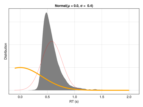
Reaction time (RTs) have been traditionally modeled using traditional linear models and their derived statistical tests such as t-test and ANOVAs. Importantly, linear models - by definition - will try to predict the mean of the outcome variable by estimating the “best fitting” Normal distribution. In the context of reaction times (RTs), this is not ideal, as RTs typically exhibit a non-normal distribution, skewed towards the left with a long tail towards the right. This means that the parameters of a Normal distribution (mean \(\mu\) and standard deviation \(\sigma\)) are not good descriptors of the data.
Linear models try to find the best fitting Normal distribution for the data. However, for reaction times, even the best fitting Normal distribution (in red) does not capture well the actual data (in grey).
A popular mitigation method to account for the non-normality of RTs is to transform the data, using for instance the popular log-transform. However, this practice should be avoided as it leads to various issues, including loss of power and distorted results interpretation (Lo and Andrews 2015; Schramm and Rouder 2019). Instead, rather than applying arbitrary data transformation, it would be better to swap the Normal distribution used by the model for a more appropriate one that can better capture the characteristics of a RT distribution.
5.5 Shifted LogNormal Model
One of the obvious candidate alternative to the log-transformation would be to use a model with a Log-transformed Normal distribution. A LogNormal distribution is a distribution of a random variable whose logarithm is normally distributed. In this model, the mean\(\mu\) and is defined on the log-scale, and effects must be interpreted as multiplicative rather than additive (the condition increases the mean RT by a factor of \(\exp(\mu_{condition})\)).
Note that for LogNormal distributions (as it is the case for many of the models introduced in the rest of the capter), the distribution parameters (\(\mu\) and \(\sigma\)) are not independent with respect to the mean and the standard deviation (SD). The empirical SD increases when the mean\(\mu\) increases (which is seen as a feature rather than a bug, as it is consistent with typical reaction time data, Wagenmakers, Grasman, and Molenaar 2005).
A Shifted LogNormal model introduces a shift (a delay) parameter tau\(\tau\) that corresponds to the minimum “starting time” of the response process.
We need to set a prior for this parameter, which is usually truncated between 0 (to exclude negative minimum times) and the minimum RT of the data (the logic being that the minimum delay for response must be lower than the faster response actually observed).
While \(Uniform(0, min(RT))\) is a common choice of prior, it is not ideal as it implies that all values between 0 and the minimum RT are equally likely, which is not the case. Indeed, psychology research has shown that such minimum response time for Humans is often betwen 100 and 250 ms. Moreover, in our case, we explicitly removed all RTs below 180 ms, suggesting that the minimum response time is more likely to approach 180 ms than 0 ms.
5.5.1 Prior on Minimum RT
Instead of a \(Uniform\) prior, we will use a \(Gamma(1.1, 11)\) distribution (truncated at min. RT), as this particular parameterization reflects the low probability of very low minimum RTs (near 0) and a steadily increasing probability for increasing times.
┌ Warning: Found `resolution` in the theme when creating a `Scene`. The `resolution` keyword for `Scene`s and `Figure`s has been deprecated. Use `Figure(; size = ...` or `Scene(; size = ...)` instead, which better reflects that this is a unitless size and not a pixel resolution. The key could also come from `set_theme!` calls or related theming functions.
└ @ Makie C:\Users\domma\.julia\packages\Makie\VRavR\src\scenes.jl:220
5.5.2 Model Specification
@modelfunctionmodel_LogNormal(rt; min_rt=minimum(df.RT), condition=nothing)# Priors τ ~truncated(Gamma(1.1, 11); upper=min_rt) μ_intercept ~Normal(0, exp(1)) # On the log-scale: exp(μ) to get value in seconds μ_condition ~Normal(0, exp(0.3)) σ_intercept ~truncated(Normal(0, 0.5); lower=0) σ_condition ~Normal(0, 0.1)for i in1:length(rt) μ = μ_intercept + μ_condition * condition[i] σ = σ_intercept + σ_condition * condition[i]if σ <0# Avoid negative variance values Turing.@addlogprob! -Infreturnnothingend rt[i] ~ShiftedLogNormal(μ, σ, τ)endendfit_LogNormal =model_LogNormal(df.RT; condition=df.Accuracy)chain_LogNormal =sample(fit_LogNormal, NUTS(), 400)
pred =predict(model_LogNormal([(missing) for i in1:length(df.RT)]; condition=df.Accuracy), chain_LogNormal)pred =Array(pred)fig =plot_distribution(df, "Predictions made by Shifted LogNormal Model")for i in1:length(chain_LogNormal)lines!(Makie.KernelDensity.kde(pred[:, i]), color=ifelse(df.Accuracy[i] ==1, "#388E3C", "#D32F2F"), alpha=0.1)endfig
┌ Warning: Found `resolution` in the theme when creating a `Scene`. The `resolution` keyword for `Scene`s and `Figure`s has been deprecated. Use `Figure(; size = ...` or `Scene(; size = ...)` instead, which better reflects that this is a unitless size and not a pixel resolution. The key could also come from `set_theme!` calls or related theming functions.
└ @ Makie C:\Users\domma\.julia\packages\Makie\VRavR\src\scenes.jl:220
This model provides a much better fit to the data, and confirms that the Accuracy condition is associated with higher RTs and higher variability (i.e., a larger distribution width).
LogNormal distributions in nature
The reason why the Normal distribution is so ubiquituous in nature (and hence used as a good default) is due to the Central Limit Theorem, which states that the sum of a large number of independent random variables will be approximately normally distributed. Because many things in nature are the result of the addition of many random processes, the Normal distribution is very common in real life.
However, it turns out that the multiplication of random variables result in a LogNormal distribution, and multiplicating (rather than additive) cascades of processes are also very common in nature, from lengths of latent periods of infectious diseases to distribution of mineral resources in the Earth’s crust, and the elemental mechanisms at stakes in physics and cell biolody (Limpert, Stahel, and Abbt 2001).
Thus, using LogNormal distributions for RTs can be justified with the assumption that response times are the result of multiplicative stochastic processes happening in the brain.
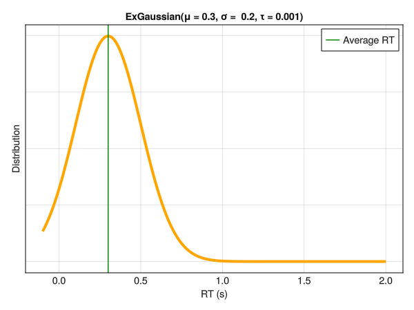
This distribution is a convolution of normal and exponential distributions and has three parameters, namely mu\(\mu\) and sigma\(\sigma\) - the mean and standard deviation of the Gaussian distribution - and tau\(\tau\) - the exponential component of the distribution (note that although denoted by the same letter, it does not correspond directly to a shift of the distribution). Intuitively, these parameters reflect the centrality, the width and the tail dominance, respectively.
Beyond the descriptive value of these types of models, some have tried to interpret their parameters in terms of cognitive mechanisms, arguing for instance that changes in the Gaussian components (\(\mu\) and \(\sigma\)) reflect changes in attentional processes [e.g., “the time required for organization and execution of the motor response”; Hohle (1965)], whereas changes in the exponential component (\(\tau\)) reflect changes in intentional (i.e., decision-related) processes (Kieffaber et al. 2006). However, Matzke and Wagenmakers (2009) demonstrate that there is likely no direct correspondence between ex-Gaussian parameters and cognitive mechanisms, and underline their value primarily as descriptive tools, rather than models of cognition per se.
Descriptively, the three parameters can be interpreted as:
Mu\(\mu\) : The location / centrality of the RTs. Would correspond to the mean in a symmetrical distribution.
Sigma\(\sigma\) : The variability and dispersion of the RTs. Akin to the standard deviation in normal distributions.
Tau\(\tau\) : Tail weight / skewness of the distribution.
Important
Note that these parameters are not independent with respect to distribution characteristics, such as the empirical mean and SD. Below is an example of different distributions with the same location (mu\(\mu\)) and dispersion (sigma\(\sigma\)) parameters. Although only the tail weight parameter (tau\(\tau\)) is changed, the whole distribution appears to shift is centre of mass. Hence, one should be careful note to interpret the values of mu\(\mu\) directly as the “mean” or the distribution peak and sigma\(\sigma\) as the SD or the “width”.
5.6.1 Conditional Tau \(\tau\) Parameter
In the same way as we modeled the effect of the condition on the variance component sigma\(\sigma\), we can do the same for any other parameters, including the exponential component tau\(\tau\). All wee need is to set a prior on the intercept and the condition effect, and make sure that \(\tau > 0\).
pred =predict(model_ExGaussian([(missing) for i in1:length(df.RT)]; condition=df.Accuracy), chain_ExGaussian)pred =Array(pred)fig =plot_distribution(df, "Predictions made by Shifted LogNormal Model")for i in1:length(chain_ExGaussian)lines!(Makie.KernelDensity.kde(pred[:, i]), color=ifelse(df.Accuracy[i] ==1, "#388E3C", "#D32F2F"), alpha=0.1)endfig
┌ Warning: Found `resolution` in the theme when creating a `Scene`. The `resolution` keyword for `Scene`s and `Figure`s has been deprecated. Use `Figure(; size = ...` or `Scene(; size = ...)` instead, which better reflects that this is a unitless size and not a pixel resolution. The key could also come from `set_theme!` calls or related theming functions.
└ @ Makie C:\Users\domma\.julia\packages\Makie\VRavR\src\scenes.jl:220
The ExGaussian model also provides an excellent fit to the data. Moreover, by modeling more parameters (including tau\(\tau\)), we can draw more nuanced conclusions. In this case, the Accuracy condition is associated with higher RTs, higher variability, and a heavier tail (i.e., more extreme values).
5.7 Shifted Wald Model
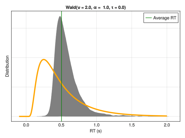
The Wald distribution, also known as the Inverse Gaussian distribution, corresponds to the distribution of the first passage time of a Wiener process with a drift rate \(\mu\) and a diffusion rate \(\sigma\). While we will unpack this definition below and emphasize its important consequences, one can first note that it has been described as a potential model for RTs when convoluted with an exponential distribution (in the same way that the ExGaussian distribution is a convolution of a Gaussian and an exponential distribution). However, this Ex-Wald model (Schwarz 2001) was shown to be less appropriate than one of its variant, the Shifted Wald distribution (Heathcote 2004; Anders et al. 2016).
Note that the Wald distribution, similarly to the models that we will be covering next (the “generative” models), is different from the previous distributions in that it is not characterized by a “location” and “scale” parameters (mu\(\mu\) and sigma\(\sigma\)). Instead, the parameters of the Shifted Wald distribution are:
Nu\(\nu\) : A drift parameter, corresponding to the strength of the evidence accumulation process.
Alpha\(\alpha\) : A threshold parameter, corresponding to the amount of evidence required to make a decision.
Tau\(\tau\) : A delay parameter, corresponding to the non-response time (i.e., the minimum time required to process the stimulus and respond). A shift parameter similar to the one in the Shifted LogNormal model.
As we can see, these parameters do not have a direct correspondence with the mean and standard deviation of the distribution. Their interpretation is more complex but, as we will see below, offers a window to a new level of interpretation.
Note
Explanations regarding these new parameters will be provided in the next chapter.
pred =predict(model_Wald([(missing) for i in1:length(df.RT)]; condition=df.Accuracy), chain_Wald)pred =Array(pred)fig =plot_distribution(df, "Predictions made by Shifted Wald Model")for i in1:length(chain_Wald)lines!(Makie.KernelDensity.kde(pred[:, i]), color=ifelse(df.Accuracy[i] ==1, "#388E3C", "#D32F2F"), alpha=0.1)endfig
┌ Warning: Found `resolution` in the theme when creating a `Scene`. The `resolution` keyword for `Scene`s and `Figure`s has been deprecated. Use `Figure(; size = ...` or `Scene(; size = ...)` instead, which better reflects that this is a unitless size and not a pixel resolution. The key could also come from `set_theme!` calls or related theming functions.
└ @ Makie C:\Users\domma\.julia\packages\Makie\VRavR\src\scenes.jl:220
5.7.2 Model Comparison
At this stage, given the multiple options avaiable to model RTs, you might be wondering which model is the best. One can compare the models using the Leave-One-Out Cross-Validation (LOO-CV) method, which is a Bayesian method to estimate the out-of-sample predictive accuracy of a model.
The loo_compare() function orders models from best to worse based on their ELPD (Expected Log Pointwise Predictive Density) and provides the difference in ELPD between the best model and the other models. As one can see, traditional linear models perform terribly.
5.8 Shifted LogNormal Mixed Model
Complex example walkthrough. Add Random effects.
Anders, Royce, F Alario, Leendert Van Maanen, et al. 2016. “The Shifted Wald Distribution for Response Time Data Analysis.”Psychological Methods 21 (3): 309.
Balota, David A, and Melvin J Yap. 2011. “Moving Beyond the Mean in Studies of Mental Chronometry: The Power of Response Time Distributional Analyses.”Current Directions in Psychological Science 20 (3): 160–66.
Heathcote, Andrew. 2004. “Fitting Wald and Ex-Wald Distributions to Response Time Data: An Example Using Functions for the s-PLUS Package.”Behavior Research Methods, Instruments, & Computers 36: 678–94.
Heathcote, Andrew, and Jonathon Love. 2012. “Linear Deterministic Accumulator Models of Simple Choice.”Frontiers in Psychology 3: 292.
Hohle, Raymond H. 1965. “Inferred Components of Reaction Times as Functions of Foreperiod Duration.”Journal of Experimental Psychology 69 (4): 382.
Kieffaber, Paul D, Emily S Kappenman, Misty Bodkins, Anantha Shekhar, Brian F O’Donnell, and William P Hetrick. 2006. “Switch and Maintenance of Task Set in Schizophrenia.”Schizophrenia Research 84 (2-3): 345–58.
Limpert, Eckhard, Werner A Stahel, and Markus Abbt. 2001. “Log-Normal Distributions Across the Sciences: Keys and Clues: On the Charms of Statistics, and How Mechanical Models Resembling Gambling Machines Offer a Link to a Handy Way to Characterize Log-Normal Distributions, Which Can Provide Deeper Insight into Variability and Probability—Normal or Log-Normal: That Is the Question.”BioScience 51 (5): 341–52.
Lo, Steson, and Sally Andrews. 2015. “To Transform or Not to Transform: Using Generalized Linear Mixed Models to Analyse Reaction Time Data.”Frontiers in Psychology 6: 1171.
Matzke, Dora, and Eric-Jan Wagenmakers. 2009. “Psychological Interpretation of the Ex-Gaussian and Shifted Wald Parameters: A Diffusion Model Analysis.”Psychonomic Bulletin & Review 16: 798–817.
Schramm, Pele, and Jeffrey N Rouder. 2019. “Are Reaction Time Transformations Really Beneficial?”
Schwarz, Wolfgang. 2001. “The Ex-Wald Distribution as a Descriptive Model of Response Times.”Behavior Research Methods, Instruments, & Computers 33: 457–69.
Thériault, Rémi, Mattan S Ben-Shachar, Indrajeet Patil, Daniel Lüdecke, Brenton M Wiernik, and Dominique Makowski. 2024. “Check Your Outliers! An Introduction to Identifying Statistical Outliers in r with Easystats.”Behavior Research Methods 56 (4): 4162–72.
Wagenmakers, Eric-Jan, Raoul PPP Grasman, and Peter CM Molenaar. 2005. “On the Relation Between the Mean and the Variance of a Diffusion Model Response Time Distribution.”Journal of Mathematical Psychology 49 (3): 195–204.
Wagenmakers, Eric-Jan, Roger Ratcliff, Pablo Gomez, and Gail McKoon. 2008. “A Diffusion Model Account of Criterion Shifts in the Lexical Decision Task.”Journal of Memory and Language 58 (1): 140–59.
Wiemann, Paul FV, Thomas Kneib, and Julien Hambuckers. 2023. “Using the Softplus Function to Construct Alternative Link Functions in Generalized Linear Models and Beyond.”Statistical Papers, 1–26.