Density, random generation, and brms custom family for the Ex-Gaussian
distribution, using the "classical" parameterization familiar to
experimental psychologists, in which mu and sigma are the mean and SD
of the Gaussian component alone, and tau is the mean of the exponential
component (the tail). This is unlike brms's built-in exgaussian()
family, in which mu indexes the mean of the entire distribution
(Gaussian + exponential components combined).
Functions:
rcogmod_exgaussian(): Simulates random draws from the Ex-Gaussian distribution.dcogmod_exgaussian(): Computes the density (likelihood) of the Ex-Gaussian distribution.pcogmod_exgaussian(): Computes the cumulative distribution function (CDF) or survival.cogmod_exgaussian(): Creates abrms::custom_family()for use inbrmsmodels.
Usage
rcogmod_exgaussian(n, mu = 0.5, sigma = 0.1, tau = 0.2)

dcogmod_exgaussian(x, mu = 0.5, sigma = 0.1, tau = 0.2, log = FALSE)

pcogmod_exgaussian(
  q,
  mu = 0.5,
  sigma = 0.1,
  tau = 0.2,
  lower.tail = TRUE,
  log.p = FALSE
)

cogmod_exgaussian(
  link_mu = "identity",
  link_sigma = "softplus",
  link_tau = "softplus"
)

cogmod_exgaussian_lpdf_expose()

cogmod_exgaussian_stanvars()

log_lik_cogmod_exgaussian(i, prep)

posterior_predict_cogmod_exgaussian(i, prep, ...)

posterior_epred_cogmod_exgaussian(prep)
Arguments
- n
Number of observations. If
length(n) > 1, the length is taken to be the number required.- mu
Mean of the Gaussian component. Unbounded - it is a location, not a scale - though for RT data it is normally positive. Range: (-Inf, Inf).
- sigma
SD of the Gaussian component. Must be positive. Range: (0, Inf).
- tau
Mean of the exponential component (the tail). Must be positive. Range: (0, Inf).
- x
Vector of quantiles (observed reaction times).
- log
Logical; if TRUE, probabilities p are given as log(p).
- q
Vector of quantiles (reaction times, in seconds).
- lower.tail
Logical; if TRUE (default), probabilities are
P[X <= q], otherwiseP[X > q]- the survival, which is what a right-censored response contributes to the likelihood underbrms::bf(rt | cens(x) ~ ...). See the Censoring section ofrcogmod_invgaussian().- log.p
Logical; if TRUE, probabilities p are given as log(p).
- link_mu, link_sigma, link_tau
Character of the type of link used to model the ex-Gaussian parameters. Defaults to
"identity"formuand"softplus"forsigmaandtau(see Details).- i, prep
For brms' functions to run: index of the observation and a
brmspreparation object.- ...
Additional arguments.
Value
rcogmod_exgaussian() returns a numeric vector of n simulated
reaction times, in seconds. dcogmod_exgaussian() returns the density at
each element of x - the log density if log = TRUE - recycled to the
length of the longest argument. pcogmod_exgaussian() returns the
cumulative probability at each element of q, honouring lower.tail and
log.p. cogmod_exgaussian() returns a
brms::custom_family object, to put on a brms::bf() formula.
cogmod_exgaussian_stanvars() returns a brms::stanvars object holding
the family's Stan functions block, to pass to brms::brm(), and
cogmod_exgaussian_lpdf_expose() compiles that Stan code and returns it
as an R function, for checking the density outside of a model. The
remaining functions are brms post-processing methods, called by brms
rather than directly: log_lik_cogmod_exgaussian() returns a numeric
vector holding one log-likelihood value per posterior draw for
observation i, posterior_predict_cogmod_exgaussian() a draws x 1
matrix of reaction times simulated for observation i, and
posterior_epred_cogmod_exgaussian() a draws x observations matrix of
expected reaction times.
Details
The Ex-Gaussian distribution is the sum of an independent Normal (Gaussian)
random variable with mean mu and SD sigma, and an Exponential random
variable with mean tau (rate 1 / tau). Unlike brms's built-in
exgaussian() family - in which mu indexes the mean of the entire
distribution (Gaussian + exponential components combined) - here mu is
the mean of the Gaussian component alone, so that the mean of the full
distribution is mu + tau.
This distinction matters because changes in the Gaussian location (mu)
and changes in the exponential tail (tau) can offset one another at the
level of the overall mean, so effects estimated on brms's default mu
can lead to different (and potentially incorrect) inferences than effects
estimated on this classical mu.
In the brms custom family (cogmod_exgaussian()), sigma and tau use a
"softplus" link (log(1 + exp(x))) rather than "log". Both are scales
and must be strictly positive for the density to exist at all. A "log" link
would enforce that too, but its curvature explodes as the linear predictor
departs from zero, producing extreme gradients and making priors and sampling
harder to calibrate - and tau is on the RT scale (seconds), where it can
take comparatively large values. "softplus" is positive-constrained like
"log" but behaves almost linearly (softplus(x) ~ x) away from zero, so
weakly-informative priors can be stated directly on the RT scale.
mu is different, and uses "identity". It is the location of the
Gaussian component, not a scale: the convolution is well defined for any real
value, and the density integrates to one at mu = 0 or below just as it does
above (the Stan lpdf has always accepted a non-positive mu - it checks
only sigma and tau). Nothing is gained by constraining it, and two things
are lost. First, interpretability, which is most of the reason to prefer the
ex-Gaussian in the first place: behind a softplus link a coefficient is not
in seconds, and the conversion factor moves with the intercept - the local
slope is 0.33 at mu = 0.4 s, 0.39 at 0.5 s and 0.63 at 1 s, so the same
effect reads as a different number depending on where the intercept sits. On
"identity" a coefficient is seconds, full stop. Second, fidelity: for fast,
heavily-tailed data the Gaussian component genuinely belongs near or below
zero with tau carrying the mass, and forcing mu > 0 distorts the mu/tau
split in exactly the cases where that decomposition is the thing being
estimated. This also matches every other implementation - brms's own
exgaussian(), retimes, and the estimates reported in the literature - so
fitted values are directly comparable.
The cost is that brms's default intercept prior is no longer sensible for
mu (student_t(3, 0, 2.5) centred at zero seconds), which is why
cogmod_priors() now supplies one.
References
Matzke, D., & Wagenmakers, E. J. (2009). Psychological interpretation of the ex-Gaussian and shifted Wald parameters: A diffusion model analysis. Psychonomic Bulletin & Review, 16(5), 798-817. doi:10.3758/PBR.16.5.798
Examples
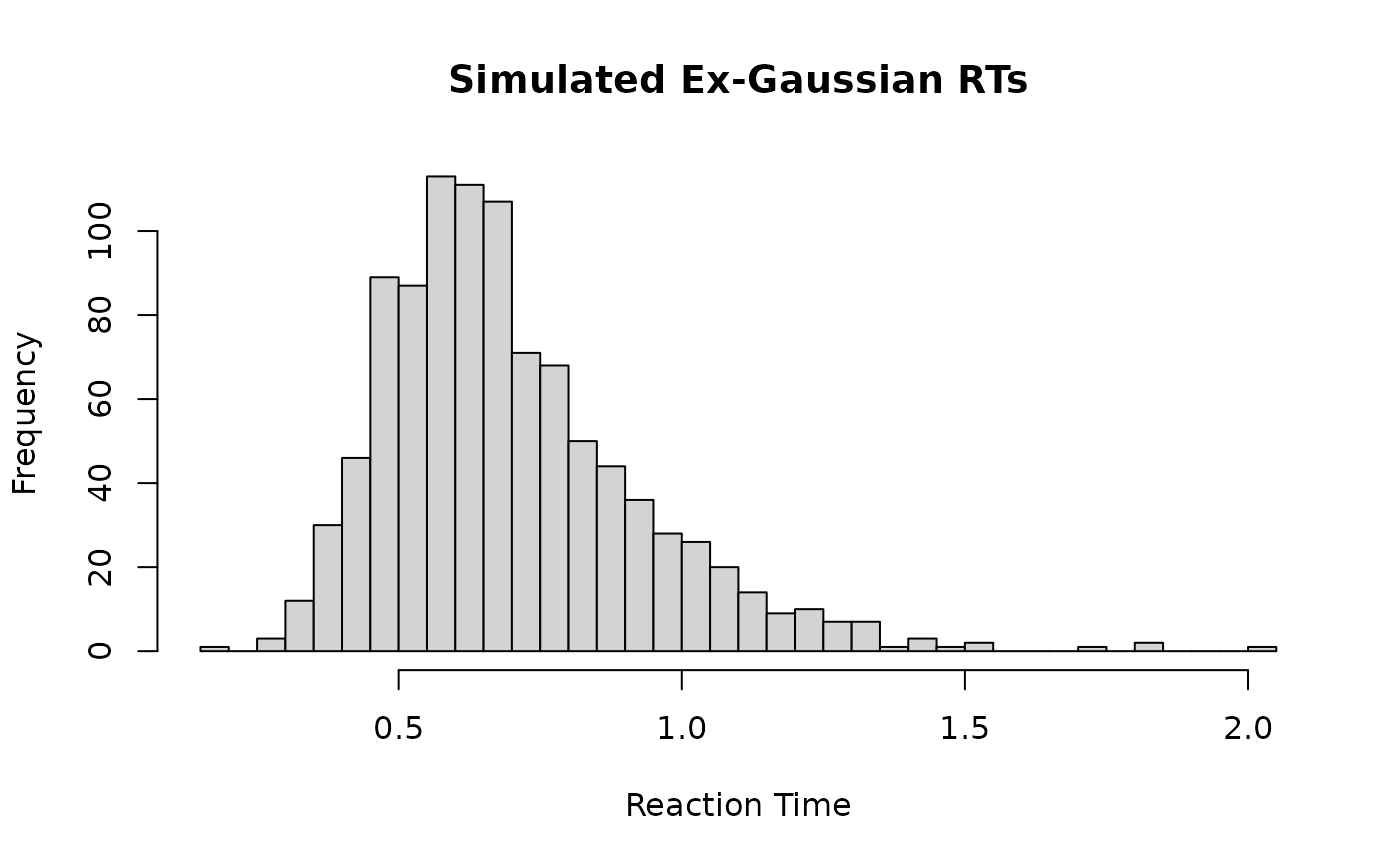
# Simulate 1000 RTs
rts <- rcogmod_exgaussian(1000, mu = 0.5, sigma = 0.1, tau = 0.2)
hist(rts, breaks = 50, main = "Simulated Ex-Gaussian RTs", xlab = "Reaction Time")