Shifted Wald Model (Inverse Gaussian)

Density, distribution function, random generation, and brms custom family for the Shifted Wald distribution, also known as the Shifted Inverse Gaussian. A Wald-distributed decision time is shifted by a non-decision time ndt, and a fixed proportion poutlier of responses is generated by an outlier process instead of by the decision process. The drift rate can be fixed across trials (the classic Wald) or drawn afresh on each one, with SD sigmadrift, and the non-decision time can be fixed or spread over a range sigmandt.

Functions:

• rcogmod_invgaussian(): Simulates random draws.

• dcogmod_invgaussian(): Computes the density (likelihood).

• pcogmod_invgaussian(): Computes the cumulative distribution function (CDF).

• cogmod_invgaussian(): Creates a brms::custom_family().

• cogmod_invgaussian_stanvars(): Generates the stanvars to pass to brm().

Usage

rcogmod_invgaussian(
  n,
  drift = 3,
  boundary = 0.5,
  ndt = 0.2,
  sigmadrift = 0,
  sigmandt = 0,
  poutlier = 0
)

dcogmod_invgaussian(
  x,
  drift = 3,
  boundary = 0.5,
  ndt = 0.2,
  sigmadrift = 0,
  sigmandt = 0,
  poutlier = 0,
  log = FALSE
)

pcogmod_invgaussian(
  q,
  drift = 3,
  boundary = 0.5,
  ndt = 0.2,
  sigmadrift = 0,
  sigmandt = 0,
  poutlier = 0,
  lower.tail = TRUE,
  log.p = FALSE
)

cogmod_invgaussian(
  link_mu = "softplus",
  link_boundary = "softplus",
  link_sigmadrift = "softplus",
  link_sigmandt = "log",
  link_ndt = "log",
  link_poutlier = "logit",
  predict_outliers = FALSE
)

cogmod_invgaussian_lpdf_expose()

cogmod_invgaussian_stanvars()

log_lik_cogmod_invgaussian(i, prep)

posterior_predict_cogmod_invgaussian(i, prep, predict_outliers = NULL, ...)

posterior_epred_cogmod_invgaussian(prep, predict_outliers = NULL)

Arguments

n

Number of observations. If length(n) > 1, the length is taken to be the number required.

drift

Drift rate. Must be positive. Represents the average speed of evidence accumulation. Range: (0, Inf).

boundary

Decision threshold (boundary separation). Must be positive. Represents the amount of evidence needed to make a decision. Range: (0, Inf).

ndt

Non-decision time (shift parameter), in seconds. Must be non-negative. Represents time for processes such as stimulus encoding and response execution. Range: [0, Inf).

sigmadrift

Between-trial SD of the drift rate. Must be non-negative. The drift of each trial is drawn from a Normal(drift, sigmadrift) truncated at zero. Default 0, which is the classic fixed-drift Wald. Range: [0, Inf).

sigmandt

Between-trial range of the non-decision time (st0), in seconds. Must be non-negative. The non-decision time of each trial is drawn from Uniform(ndt, ndt + sigmandt), so ndt is its lower bound. Default 0, a fixed non-decision time. Range: [0, Inf).

poutlier

Proportion of responses generated by the outlier process rather than by the decision process. Range: [0, 1]. At poutlier = 0 the distribution reduces to the plain shifted LogNormal.

x

Vector of quantiles (observed reaction times).

log

Logical; if TRUE, probabilities p are given as log(p).

q

Vector of quantiles (observed reaction times).

lower.tail

Logical; if TRUE (default), probabilities are P[X <= x], otherwise P[X > x].

log.p

Logical; if TRUE, probabilities p are given as log(p).

link_mu, link_boundary, link_sigmadrift, link_sigmandt, link_ndt, link_poutlier

Link functions for the parameters. mu is the drift rate. sigmadrift and sigmandt are legitimately zero, which is the classic Wald, and are fixed there by writing sigmadrift = 0 and sigmandt = 0 in the formula. sigmandt is on a log link, as cogmod_ddm()'s is: it is the same quantity in the same unit, and at the tens of milliseconds it lives at a log and a softplus link agree to within a few percent, so what decides it is that a normal prior on the log scale is exactly a lognormal on the natural one, and the prior means the same thing whether or not the parameter is written in bf().

predict_outliers

Logical; whether posterior_predict() and posterior_epred() should include the outlier component. FALSE (the default) fixes poutlier to zero for prediction, so predictions describe the decision process alone; the likelihood is always the full mixture either way. See with_outliers().

i, prep

For brms' functions to run: index of the observation and a brms preparation object.

...

Additional arguments.

Value

rcogmod_invgaussian() returns a numeric vector of n simulated reaction times, in seconds. dcogmod_invgaussian() returns the density at each element of x - the log density if log = TRUE - recycled to the length of the longest argument. pcogmod_invgaussian() returns the cumulative probability at each element of q, honouring lower.tail and log.p. cogmod_invgaussian() returns a brms::custom_family object, to put on a brms::bf() formula. cogmod_invgaussian_stanvars() returns a brms::stanvars object holding the family's Stan functions block, to pass to brms::brm(), and cogmod_invgaussian_lpdf_expose() compiles that Stan code and returns it as an R function, for checking the density outside of a model. The remaining functions are brms post-processing methods, called by brms rather than directly: log_lik_cogmod_invgaussian() returns a numeric vector holding one log-likelihood value per posterior draw for observation i, and posterior_predict_cogmod_invgaussian() a draws x 1 matrix of reaction times simulated for observation i. posterior_epred_cogmod_invgaussian() returns a draws x observations matrix of expected reaction times, with Inf wherever the mean does not exist.

Details

The Wald distribution describes the time it takes for a Wiener diffusion process starting at 0 to reach a threshold boundary > 0, given a positive drift rate drift > 0. That time is then shifted by a non-decision time ndt.

It is mathematically equivalent to shifting an Inverse Gaussian distribution with mean boundary / drift and shape boundary^2. In the brms family the drift rate is named mu, since brms requires a parameter of that name.

ndt and poutlier mean exactly what they do in cogmod_lognormal(), and with_outliers(), without_outliers(), p_outlier() and cogmod_priors() all work here too. See ?rcogmod_lognormal for why ndt is expressed directly in seconds rather than as a fraction of the fastest observed response, what the half Normal outlier component is for, and why the outlier component's scale is a constant rather than a dpar, and why reaction times have to be in seconds.

The Wald density vanishes at the shift with all derivatives, like the LogNormal, so ndt is well behaved here and there is no unbounded-likelihood boundary of the kind cogmod_gamma() and cogmod_weibull() have at shape < 1.

The random generation algorithm is that of Michael, Schucany, and Haas (1976), as used in the statmod package.

Across-trial drift variability

sigmadrift is the between-trial SD of the drift rate. At sigmadrift = 0, its default, every trial accumulates at the same rate and the model is the classic Wald. Above zero, each trial draws its own drift from a Normal(mu, sigmadrift) truncated at zero, which is what lets the model produce the long right tails empirical RT distributions have, and is the single-accumulator counterpart of what cogmod_ddm() calls sigmadrift and cogmod_lba1() calls sigma. Marginalising over that draw is a Gaussian integral, so the density stays closed form and costs two normal CDFs.

The truncation matters. A single-boundary accumulator handed a negative drift never terminates, so an untruncated Normal would leave the density defective: it integrates to 0.99 at mu = 3, boundary = 0.5, sigmadrift = 1.5, and to 0.69 at mu = 0.5, boundary = 1, sigmadrift = 2. cogmod_ddm() needs no such truncation, a diffusion between two boundaries always absorbing at one of them.

In a formula, sigmadrift = 0 fixes the parameter and gives the classic Wald; leaving it out of bf() altogether estimates it, which is not the same thing:

# Classic Wald
brms::bf(rt ~ 1, boundary ~ 1, sigmadrift = 0, sigmandt = 0, ndt ~ 1,
         poutlier ~ 1, family = cogmod_invgaussian())

# With across-trial drift variability
brms::bf(rt ~ 1, boundary ~ 1, sigmadrift ~ 1, sigmandt = 0, ndt ~ 1,
         poutlier ~ 1, family = cogmod_invgaussian())

Fixing it is the better default, for two reasons. sigmadrift and poutlier both fatten the right tail and are only weakly distinguishable: on 2000 simulated trials at mu = 3, boundary = 0.5, sigmadrift = 0.8, estimating sigmadrift buys about 2 log-likelihood units over fixing it at zero, and the outlier weight absorbs most of the difference. And scaling mu, boundary and sigmadrift up by a common factor sends the Wald to the reciprocal-normal (LATER) limit, where the within-trial noise stops mattering and RT = boundary / drift exactly - so large values of all three describe nearly the same distribution. cogmod_priors() gives sigmadrift a deliberately informative prior to fence off both.

One consequence is worth stating plainly: with sigmadrift > 0 the density decays as t^-2, because drifts arbitrarily close to zero take arbitrarily long, so the mean does not exist. posterior_epred() returns Inf, as it does for cogmod_invgamma() at shape <= 1. Use posterior_predict() and summarise the draws with a median or a quantile instead.

Across-trial non-decision time variability

sigmandt is the between-trial range of the non-decision time, st0 in the usual notation, and the single-boundary counterpart of cogmod_ddm()'s sigmandt. At sigmandt = 0, its default, every trial has the same non-decision time ndt. Above zero each trial draws its own from Uniform(ndt, ndt + sigmandt), so ndt becomes the lower bound of the non-decision time and the leading edge of the distribution is spread over an interval instead of starting sharply. Averaging the shift out turns the density into a difference of two Wald CDFs and the CDF into a difference of two integrated CDFs, and for the Wald both are closed form, so the parameter costs a handful of normal CDFs per observation and cens() works with it unchanged. With sigmadrift > 0 as well, everything is taken by the same quadrature over the drift that the CDF already uses.

It is hard to estimate, and for most applications should be fixed at zero. Three parameters shape the leading edge of the distribution: ndt places it, sigmandt smears it and poutlier puts mass in front of it, and they trade off against one another on any dataset without a sharp onset. st0 is also the parameter the DDM literature agrees is recovered worst. Estimate it only with a lot of data, a strong prior, or both - cogmod_priors() gives it the same deliberately tight prior as cogmod_ddm()'s - and otherwise write sigmandt = 0 in bf(), which removes it from the model altogether. As with sigmadrift, leaving it out of bf() estimates it.

Censoring: errors, timeouts and omissions

brms's cens() addition term works on this family:

brms::bf(rt | cens(error) ~ condition, boundary ~ condition, ndt ~ 1,
         sigmadrift = 0, sigmandt = 0, family = cogmod_invgaussian())

A trial with error = 1 (or TRUE, or "right") is then a right-censored correct response: its RT is read as a lower bound on when the correct process would have finished, and it contributes the survival P(T > rt) to the likelihood where an observed response contributes the density. With sigmadrift = 0 this is the censored shifted Wald of Miller et al. (2018), the cswald model of the bmm package. Here it is not a separate family but a construction: no new parameter, no new syntax, and the same cens() works on every RT-only family with a closed-form CDF (see ?rcogmod_lognormal). Left-censoring (error = -1 or "left") and interval-censoring (cens(x, y2)) work the same way, and log_lik() - hence loo() - honours all three.

Three things follow from the construction:

• What it is for. A two-accumulator race has to estimate an error process, and when errors are few that process is identified by nothing; see the driftone discussion in cogmod_rdm(). Censoring has no error accumulator to run away, uses the errors' timing instead of discarding the trials, and is exactly right - not an approximation - for go/no-go, deadline and omission designs, where a non-response genuinely is a censored draw from one accumulator.

• What it assumes. That an error says nothing about the correct process beyond "not finished yet": non-informative censoring. That is false wherever errors and correct responses come from one evidence path, which is the DDM's picture, and cogmod_priors() warns past 20% censored trials, well beyond the high-accuracy regime the model is argued for.

• The check to run first. Censoring draws errors from the surviving tail, so it can only ever predict them slower than correct responses. Fast errors - a low boundary, a biased start point - are unproducible by construction. Compare the two RT distributions before fitting; if errors are faster, use a race (cogmod_rdm(), cogmod_lba2(), cogmod_ddm()).

posterior_predict() predicts the latent, uncensored reaction time, as brms does for its own families, so pp_check() on a censored fit compares uncensored replicates against data whose censored rows hold censoring times. pcogmod_invgaussian(lower.tail = FALSE) is the survival a censored trial contributes, and the Stan cogmod_invgaussian_lccdf() in cogmod_invgaussian_stanvars() is its counterpart; with sigmadrift > 0 both take the CDF by quadrature over the drift, the marginal having no closed form. sigmandt > 0 changes neither: the smeared CDF and survival are closed form at a fixed drift and go through the same quadrature otherwise.

References

• Michael, J. R., Schucany, W. R., & Haas, R. W. (1976). Generating Random Variates Using Transformations with Multiple Roots. The American Statistician, 30(2), 88-90. doi:10.2307/2683801

• Anders, R., Alario, F., & Van Maanen, L. (2016). The shifted Wald distribution for response time data analysis. Psychological Methods, 21(3), 309-327. doi:10.1037/met0000063

• Matzke, D., & Wagenmakers, E. J. (2009). Psychological interpretation of the ex-Gaussian and shifted Wald parameters: A diffusion model analysis. Psychonomic Bulletin & Review, 16(5), 798-817. doi:10.3758/PBR.16.5.798

• Folks, J. L., & Chhikara, R. S. (1978). The inverse Gaussian distribution and its statistical application-a review. Journal of the Royal Statistical Society Series B: Statistical Methodology, 40(3), 263-275.

• Tillman, G., Van Zandt, T., & Logan, G. D. (2020). Sequential sampling models without random between-trial variability: The racing diffusion model of speeded decision making. Psychonomic Bulletin & Review, 27(5), 911-936. doi:10.3758/s13423-020-01719-6

• Miller, R., Scherbaum, S., Heck, D. W., Goschke, T., & Enge, S. (2018). On the relation between the (censored) shifted Wald and the Wiener distribution as measurement models for choice response times. Applied Psychological Measurement, 42(2), 116-135. doi:10.1177/0146621617710465

Examples

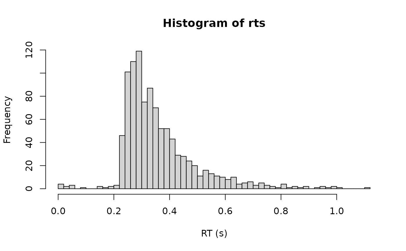
# Simulate 1000 RTs with 2% outliers
rts <- rcogmod_invgaussian(1000, drift = 3, boundary = 0.5, ndt = 0.2, poutlier = 0.02)
hist(rts, breaks = 50, xlab = "RT (s)")


# The same, with the drift varying across trials: a longer right tail
rts_sv <- rcogmod_invgaussian(1000, drift = 3, boundary = 0.5, ndt = 0.2,
                              sigmadrift = 1, poutlier = 0.02)
quantile(rts, c(0.5, 0.99))
#>       50%       99% 
#> 0.3260508 0.8664158 
quantile(rts_sv, c(0.5, 0.99))
#>       50%       99% 
#> 0.3227368 1.2222166 

# Responses faster than ndt keep positive density, unlike the unmixed model
dcogmod_invgaussian(0.1, ndt = 0.3, poutlier = 0.02)
#> [1] 0.07041307
dcogmod_invgaussian(0.1, ndt = 0.3, poutlier = 0)
#> [1] 0

# A non-decision time spread over [0.2, 0.3] s smears the leading edge
x <- seq(0.2, 0.5, by = 0.05)
rbind(fixed = dcogmod_invgaussian(x, ndt = 0.2),
      spread = dcogmod_invgaussian(x, ndt = 0.2, sigmandt = 0.1))
#>        [,1]     [,2]     [,3]     [,4]     [,5]     [,6]      [,7]
#> fixed     0 5.241002 5.164415 3.405054 2.175092 1.408261 0.9297931
#> spread    0 0.954229 3.781531 4.955366 3.499730 2.252275 1.4559368