Shifted Single-Accumulator LBA Model

Density, random generation, and brms custom family for a single-accumulator Linear Ballistic Accumulator. Evidence rises linearly and ballistically - no within-trial noise - from a start point drawn uniformly on [0, sigmabias] at a rate drawn from a normal truncated at zero, until it reaches the threshold b = sigmabias + boundary. That finishing time is shifted by a non-decision time ndt, and a fixed proportion poutlier of responses is generated by an outlier process instead.

Fixing sigmabias = 0 gives the recinormal, or LATER, model, in which 1 / (RT - ndt) is normally distributed; see the section below.

Functions:

• rcogmod_lba1(): Simulates random draws.

• dcogmod_lba1(): Computes the density (likelihood).

• cogmod_lba1(): Creates a brms::custom_family().

• cogmod_lba1_stanvars(): Generates the stanvars to pass to brm().

Usage

rcogmod_lba1(
  n,
  drift = 3,
  sigma = 1,
  sigmabias = 0.5,
  boundary = 0.5,
  ndt = 0.3,
  poutlier = 0
)

dcogmod_lba1(
  x,
  drift = 3,
  sigma = 1,
  sigmabias = 0.5,
  boundary = 0.5,
  ndt = 0.3,
  poutlier = 0,
  log = FALSE
)

cogmod_lba1(
  link_mu = "softplus",
  link_sigma = "softplus",
  link_sigmabias = "softplus",
  link_boundary = "softplus",
  link_ndt = "log",
  link_poutlier = "logit",
  predict_outliers = FALSE
)

cogmod_lba1_lpdf_expose()

cogmod_lba1_stanvars()

log_lik_cogmod_lba1(i, prep)

posterior_predict_cogmod_lba1(i, prep, predict_outliers = NULL, ...)

posterior_epred_cogmod_lba1(prep, predict_outliers = NULL)

Arguments

n

Number of observations. If length(n) > 1, the length is taken to be the number required.

drift

Mean drift rate.

sigma

Standard deviation of the drift rate. Conventionally fixed to 1.

sigmabias

The starting-point range (A); must be non-negative. Zero is the recinormal (LATER) model rather than an invalid value - see the section above.

boundary

The threshold offset, such that b = sigmabias + boundary; must be positive.

ndt

Non-decision time (shift parameter), in seconds. Must be non-negative. Represents time for processes such as stimulus encoding and response execution. Range: [0, Inf).

poutlier

Proportion of responses generated by the outlier process rather than by the decision process. Range: [0, 1]. At poutlier = 0 the distribution reduces to the plain shifted LogNormal.

x

Vector of quantiles (observed reaction times).

log

Logical; if TRUE, probabilities p are given as log(p).

link_mu, link_sigma, link_sigmabias, link_boundary, link_ndt, link_poutlier

Link functions for the parameters.

predict_outliers

Logical; whether posterior_predict() should include the outlier component. FALSE (the default) fixes poutlier to zero for prediction, so predictions describe the decision process alone; the likelihood is always the full mixture either way. See with_outliers().

i, prep

For brms' functions to run: index of the observation and a brms preparation object.

...

Additional arguments.

Value

rcogmod_lba1() returns a numeric vector of n simulated reaction times, in seconds. dcogmod_lba1() returns the density at each element of x - the log density if log = TRUE - recycled to the length of the longest argument. cogmod_lba1() returns a brms::custom_family object, to put on a brms::bf() formula. cogmod_lba1_stanvars() returns a brms::stanvars object holding the family's Stan functions block, to pass to brms::brm(), and cogmod_lba1_lpdf_expose() compiles that Stan code and returns it as an R function, for checking the density outside of a model. The remaining functions are brms post-processing methods, called by brms rather than directly: log_lik_cogmod_lba1() returns a numeric vector holding one log-likelihood value per posterior draw for observation i, and posterior_predict_cogmod_lba1() a draws x 1 matrix of reaction times simulated for observation i. posterior_epred_cogmod_lba1() returns nothing: the decision time has no finite mean, so it errors rather than report one - summarise posterior_predict() draws instead.

Details

The full LBA is a race between one accumulator per response option, with the winner determining both the choice and the RT. With no choice to model there is nothing to race, so this is the single-accumulator version and the RT is just that one accumulator's finishing time. All the RT variability comes from across-trial variability in the start point and the drift rate, rather than from moment-to-moment noise within the trial.

The threshold is written as an offset, b = sigmabias + boundary, which is the B parameterization of DMC and EMC2 (b = B + A) rather than the absolute threshold rtdists estimates. The threshold has to sit above the highest possible starting point, and the offset makes b > sigmabias hold automatically for any positive value instead of needing an order constraint between two estimated parameters. See cogmod_lba2() for the full note. The cost is that boundary alone is not the quantity to read off a fitted model; boundary + sigmabias is.

sigma is conventionally fixed to 1 rather than estimated, because the evidence scale is arbitrary: multiplying mu, sigma, sigmabias and boundary by a common constant leaves the decision time (b - start) / drift unchanged, so only ratios are identified and one parameter must be pinned at a non-zero value to fix the scale. Fix it in the formula with sigma = 1.

The recinormal (LATER) special case

Setting sigmabias = 0 removes the start-point variability altogether: the accumulator starts at zero on every trial, the decision time is b / drift, and 1 / (RT - ndt) is therefore normally distributed. That is the recinormal, better known in the oculomotor literature as the LATER model of Carpenter and Williams (1995), whose mu and sigma are the mean and SD of promptness - the quantity a reciprobit plot puts on its axis.

This is not an approximation reached in the limit. At sigmabias = 0 the density evaluates to dnorm(b / t, drift, sigma) * b / t^2 / pnorm(drift / sigma) exactly, to machine precision, in both the R and the Stan implementation. Two pins are needed rather than one, because zero is the one value the arbitrary evidence scale leaves alone and so sigmabias drops off the scale ray rather than pinning it:

# free: mu and sigma, the mean and SD of promptness
bf(rt ~ 1, sigmabias = 0, boundary = 1)

Because sigmabias is then a constant rather than a parameter, none of the trouble described next applies to it, and cogmod_priors() emits no row for it.

Estimating the start-point range

Left free, sigmabias is estimable but treacherous, precisely because the recinormal limit above is reached smoothly: once the start-point range is small enough, making it smaller stops changing the density, so the likelihood goes flat. On a softplus link zero is at minus infinity, so a flat prior there leaves the posterior improper, and the symptom is a chain that wanders off rather than one that fails. Fitted without priors on the 4285-trial data in vignette("rt_models"), sigmabias for one condition ran to softplus(-10.4) = 3e-05 with Rhat 1.69 and an effective sample size of 6.

There are two ways out, and the choice is a modelling decision rather than a technical one. Pin sigmabias = 0 and fit the recinormal, which is the honest option when the design cannot identify a start-point range. Or keep it free and fence the flat direction off with a prior: cogmod_priors() does this for both sigmabias and boundary - the threshold is b = sigmabias + boundary, so the two share the ridge - in the same way and for the same reason it fences off ndt and poutlier. Pass prior = cogmod_priors(f, df); the defaults are weak (normal(0, 1) on the softplus scale, so a start-point range of roughly 0.3 to 1.3) and are meant to be replaced rather than relied on if you know more. The two are nested, so loo_compare() on the two fits is a like-for-like comparison through the same likelihood.

ndt and poutlier mean exactly what they do in cogmod_lognormal(), and with_outliers(), without_outliers() and cogmod_priors() work here too. See ?rcogmod_lognormal for the full account.

Note that posterior_epred() is not available: the decision time has no finite mean, because E[1 / drift] diverges for a normal truncated at zero.

References

Carpenter, R. H. S., & Williams, M. L. L. (1995). Neural computation of log likelihood in control of saccadic eye movements. Nature, 377(6544), 59-62.

Examples

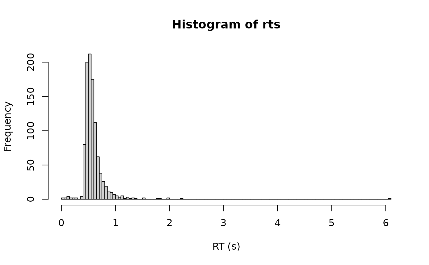
# Simulate 1000 trials with 2% outliers
rts <- rcogmod_lba1(1000, drift = 3, sigma = 1, sigmabias = 0.5, boundary = 0.5,
               ndt = 0.3, poutlier = 0.02)
hist(rts, breaks = 100, xlab = "RT (s)")


# sigmabias = 0 is the recinormal (LATER): 1 / (RT - ndt) is normal
dcogmod_lba1(0.5, drift = 3, sigma = 1, sigmabias = 0, boundary = 0.5, ndt = 0.2)
#> [1] 0.9123987
dnorm(0.5 / 0.3, 3, 1) * 0.5 / 0.3^2 / pnorm(3)
#> [1] 0.9123987

# Responses faster than ndt keep positive density, unlike the unmixed model
dcogmod_lba1(0.1, ndt = 0.3, poutlier = 0.02)
#> [1] 0.07041307
dcogmod_lba1(0.1, ndt = 0.3, poutlier = 0)
#> [1] 0