Density, random generation, and brms custom family for the shifted LogNormal
distribution. A LogNormal-distributed decision time is shifted by a
non-decision time ndt, and a fixed proportion poutlier of responses is
generated by an outlier process instead of by the decision process.
Functions:
rcogmod_lognormal(): Simulates random draws from the shifted LogNormal model.dcogmod_lognormal(): Computes the density (likelihood).pcogmod_lognormal(): Computes the cumulative distribution function (CDF) or survival.cogmod_lognormal(): Creates abrms::custom_family()for use inbrmsmodels.cogmod_lognormal_stanvars(): Generates thestanvarsto pass tobrm().p_outlier(): Per-trial posterior probability of being an outlier.
Usage
rcogmod_lognormal(
  n,
  mu = -0.7,
  sigma = 0.5,
  ndt = 0.2,
  sigmabias = 0,
  poutlier = 0
)

dcogmod_lognormal(
  x,
  mu = -0.7,
  sigma = 0.5,
  ndt = 0.2,
  sigmabias = 0,
  poutlier = 0,
  log = FALSE
)

pcogmod_lognormal(
  q,
  mu = -0.7,
  sigma = 0.5,
  ndt = 0.2,
  sigmabias = 0,
  poutlier = 0,
  lower.tail = TRUE,
  log.p = FALSE
)

cogmod_lognormal(
  link_mu = "identity",
  link_sigma = "softplus",
  link_sigmabias = "softplus",
  link_ndt = "log",
  link_poutlier = "logit",
  predict_outliers = FALSE
)

cogmod_lognormal_lpdf_expose()

cogmod_lognormal_stanvars()

log_lik_cogmod_lognormal(i, prep)

posterior_predict_cogmod_lognormal(i, prep, predict_outliers = NULL, ...)

posterior_epred_cogmod_lognormal(prep, predict_outliers = NULL)
Arguments
- n
Number of observations. If
length(n) > 1, the length is taken to be the number required.- mu
Mean of the decision time on the log scale (
meanlog). Can take any real value. Range: (-Inf, Inf).- sigma
SD of the decision time on the log scale (
sdlog). Must be positive. Range: (0, Inf).- ndt
Non-decision time (shift parameter), in seconds. Must be non-negative. Represents time for processes such as stimulus encoding and response execution. Range: [0, Inf).
- sigmabias
Start-point range, in units of the threshold offset: the decision time is the LogNormal multiplied by a
Uniform(1, 1 + sigmabias)distance. Must be non-negative. At0(the default) the model is the plain shifted LogNormal; see the section on the start-point range.- poutlier
Proportion of responses generated by the outlier process rather than by the decision process. Range:
[0, 1]. Atpoutlier = 0the distribution reduces to the plain shifted LogNormal.- x
Vector of quantiles (observed reaction times).
- log
Logical; if TRUE, probabilities p are given as log(p).
- q
Vector of quantiles (reaction times, in seconds).
- lower.tail
Logical; if TRUE (default), probabilities are
P[X <= q], otherwiseP[X > q]- the survival, which is what a right-censored response contributes to the likelihood (see the Censoring section).- log.p
Logical; if TRUE, probabilities p are given as log(p).
- link_mu, link_sigma, link_sigmabias, link_ndt, link_poutlier
Link functions for the parameters.
sigmabiasis on softplus, so that the natural-scale value reaches zero only at minus infinity - see the section on the start-point range for why it is best fixed at zero in the formula rather than estimated.- predict_outliers
Logical; whether
posterior_predict()andposterior_epred()should include the outlier component.FALSE(the default incogmod_lognormal()) fixespoutlierto zero for prediction, so predictions describe the decision process alone; the likelihood is always the full mixture either way. On the prediction methods themselves the default isNULL, which defers to the flag carried on the model - seewith_outliers()to change it after fitting. See Details.- i, prep
For brms' functions to run: index of the observation and a
brmspreparation object.- ...
Additional arguments.
Value
rcogmod_lognormal() returns a numeric vector of n simulated
reaction times, in seconds. dcogmod_lognormal() returns the density at
each element of x - the log density if log = TRUE - recycled to the
length of the longest argument. pcogmod_lognormal() returns the
cumulative probability at each element of q, honouring lower.tail and
log.p. cogmod_lognormal() returns a
brms::custom_family object, to put on a brms::bf() formula.
cogmod_lognormal_stanvars() returns a brms::stanvars object holding
the family's Stan functions block, to pass to brms::brm(), and
cogmod_lognormal_lpdf_expose() compiles that Stan code and returns it
as an R function, for checking the density outside of a model. The
remaining functions are brms post-processing methods, called by brms
rather than directly: log_lik_cogmod_lognormal() returns a numeric
vector holding one log-likelihood value per posterior draw for
observation i, and posterior_predict_cogmod_lognormal() a draws x 1
matrix of reaction times simulated for observation i.
posterior_epred_cogmod_lognormal() returns a draws x observations
matrix of expected reaction times.
Parameterization
The observed reaction time is ndt + LogNormal(mu, sigma), so mu and
sigma are the mean and SD of the decision time on the log scale, and the
median reaction time is ndt + exp(mu). That holds at sigmabias = 0, the
default of rcogmod_lognormal(), dcogmod_lognormal() and
pcogmod_lognormal() and the value to fix in the formula unless the design
can identify a start-point range; see the next section for what a positive
sigmabias adds.
The start-point range
The shifted LogNormal is a single-accumulator LBA (cogmod_lba1()) with a
LogNormal rather than truncated-Normal rate and no start-point variability:
evidence runs from zero to a threshold at a rate v ~ LogNormal(-mu, sigma),
and the finishing time 1 / v is LogNormal(mu, sigma). sigmabias puts
the start point back. Each trial starts at z ~ Uniform(0, sigmabias) and
runs to the threshold 1 + sigmabias, so the decision time is the LogNormal
multiplied by a Uniform(1, 1 + sigmabias) distance:
A Uniform distance compresses the fast tail and blunts the mode without
touching the slow tail, a shape the LogNormal alone cannot produce. The same
accumulator, raced against a second one, is cogmod_lnr(), whose nu is
-mu; the two families share their kernels and their sigmabias.
The threshold offset above the highest start point is pinned at 1, the
LBA's boundary convention with boundary = 1. It has to be the threshold
rather than sigma that pins the evidence scale: rescaling the evidence axis
shifts the rate's location and scales sigmabias and the threshold but
leaves a LogNormal rate's sigma untouched, so sigma = 1 would fix
nothing. sigmabias is therefore read in units of that offset: sigmabias = 1 says the start point varies over as wide a band as the one above it.
Estimating sigmabias is treacherous in the same way as in cogmod_lba1().
As it approaches zero the likelihood goes flat - the model is converging to
the LogNormal and once the range is small enough making it smaller changes
nothing - while the softplus link reaches zero only at minus infinity. Left
flat that is an improper posterior; cogmod_priors() fences it. On RT-only
data the range is identified through shape alone, more weakly than in the
race where accuracy helps, and the general density costs about four normal
CDFs where the LogNormal costs one. Fix sigmabias = 0 in the formula unless
the design speaks to start-point variability; at zero the family computes
exactly what it computed before the parameter existed, at the same cost.
Neither cogmod_logstudent() nor cogmod_loggamma() has a sigmabias: the
density needs a partial first moment of the rate distribution, which does not
exist for a Student-t on the log scale and needs incomplete gamma functions
for the log-Gamma.
ndt is expressed directly, in seconds (through a log link in the brms
family). Nothing about it is taken from the data: it is not bounded by the
fastest observed response, so a non-decision time that varies by condition or
by participant can exceed the sample minimum wherever the data support it.
The outlier component
A shifted distribution assigns exactly zero density to any response faster
than ndt, which puts a hard boundary in the likelihood at the fastest
observed RT. Mixing in a component with support over the whole positive line
removes it: every response keeps positive density whatever ndt is, so the
boundary becomes a finite cost rather than a wall and the log-density stays
smooth and differentiable. That is what makes the direct parameterization of
ndt workable without taking a bound from the data.
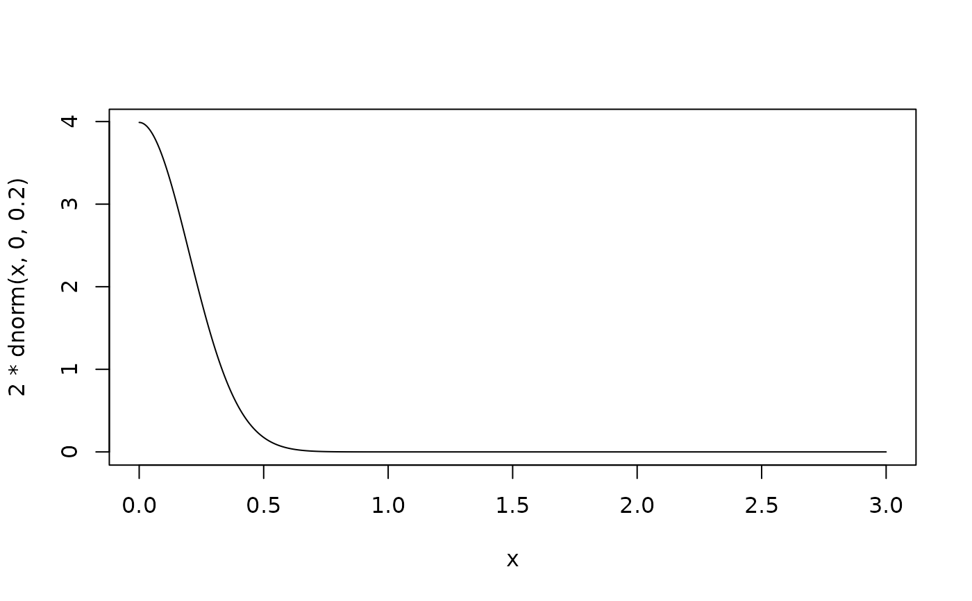
The outlier component is a half Normal with scale 0.2 seconds, i.e.
2 * dnorm(x, 0, 0.2) on [0, Inf). Two properties motivate the shape. It
is flat at the origin (zero derivative), so the very fastest responses -
the ones least plausibly decisions - are not starved of density; a LogNormal
or Gamma vanishes at zero and an Exponential peaks there with maximal slope,
and all three get this backwards. And it stays close to flat across the
whole range ndt plausibly occupies - 76% of its peak at 0.15 s and 46% at
0.25 s - while dying fast enough above that to leave the slow tail alone.
Plot it with curve(2 * dnorm(x, 0, 0.2), 0, 3).
A heavier-tailed component would not do. A half Student-t with 3 degrees of
freedom, say, has a heavier tail than every decision density in the package,
so far-out slow responses would eventually be better explained by the
outlier component than by the model: at poutlier = 0.02 a 5 s response
would be attributed to it with probability 0.86, and ndt pulled up behind
it. The slow tail belongs to the decision family, which is what
cogmod_loggamma()'s shape and cogmod_invgaussian()'s sigmadrift are
for.
Reaction times must be in seconds
The outlier component's scale is a constant in seconds, and so are the
priors cogmod_priors() supplies - ndt centred on 0.30 s,
sigmandt in cogmod_ddm() at 0.05 s, and so on. There is no argument for
changing the unit, and no unit conversion anywhere in the package.
Feeding it milliseconds fails silently, which is worth knowing about.
The outlier component's log-density at RT = 400 is about -2e6, so it
contributes nothing anywhere in the data and the mixture collapses to the
unmixed shifted family: poutlier goes to zero and ndt is pinned by the
fastest observed response again - exactly the min-RT boundary this
parameterization exists to remove. Nothing errors, and the chains still
initialise, because the decision density itself stays finite.
A scale argument in the unit of the data would make the likelihood
equivariant to that unit, and there deliberately is none: the equivariance
would be lost again in the priors, which are stated in seconds throughout,
and cogmod_priors() is not optional.
Divide by 1000 before fitting, and multiply ndt back afterwards if you
want the answer in milliseconds.
poutlier is a rate, not a classification: the model never labels
individual trials, it estimates what share of them came from elsewhere. Use
p_outlier() for per-trial posterior probabilities.
Trimmed data: pin poutlier down, but not to zero
poutlier is only weakly identified when there is little to identify it
from - which is why cogmod_priors() gives it an informative prior rather
than leaving it flat. If the data have already been trimmed, or only a
handful of implausibly fast responses remain, it is reasonable to stop asking
the data to estimate a rate at all.
The right way to do that is a very tight prior near zero, not a hard zero:
f <- brms::bf(RT ~ 1, sigma ~ 1, ndt ~ 1, poutlier ~ 1,
              family = cogmod_lognormal())
priors <- c(
  cogmod_priors(f, df),
  brms::prior(normal(-7, 0.5), class = "Intercept", dpar = "poutlier"),
  replace = TRUE
)
normal(-7, 0.5) on the logit scale is centred at about 0.09%, with 95% of
its mass between 0.03% and 0.24% - small enough to assert "there is
essentially no contamination here", while leaving the rate free to rise if
the data insist.
Fixing it outright is also possible, with poutlier = 0 in the bf(), which
makes brms treat it as a constant and reduces the model to the plain
shifted family. Prefer the tight prior. At exactly zero the density is
once again exactly zero below ndt, so the hard min-RT boundary returns and
ndt is pinned by the fastest observed response - which is the very problem
the outlier component was introduced to solve, reintroduced deliberately. A
rate of 0.1% is numerically negligible for every other purpose but still
keeps the density positive below ndt, so the likelihood stays smooth and
ndt stays free.
Trim first either way. Neither option makes slow contaminants safe: those are
confounded with the right tail and bias ndt upward, so filter them before
fitting.
Slow outliers are deliberately not handled by this component. A slow
contaminant is statistically confounded with the right tail of the RT
distribution itself, so it cannot be identified, and leaving such trials in
the data biases ndt upward. Filter implausibly slow responses before
fitting.
Predictions exclude the outlier component
posterior_predict() and posterior_epred() describe the decision process
alone by default, as if poutlier were zero. For visualising effects the
outlier component is a nuisance that pulls expected values toward its own mean
and adds a spike of implausibly fast draws; it is also a fixed regularizer
rather than a claim about how guesses are distributed, so simulating from it
means simulating from something the model does not assert.
brms::posterior_epred(m)
modelbased::estimate_means(m, by = "Condition")
marginaleffects::avg_predictions(m, by = "Condition")
Use with_outliers() for the fitted mixture, and without_outliers() to go
back. The one case that genuinely wants the mixture is a posterior predictive
check, since on untrimmed data the decision-only predictive has no fast spike
to match the one in the data:
brms::pp_check(with_outliers(m))The same flag can be set up front, with cogmod_lognormal(predict_outliers = TRUE).
The flag is carried on the model rather than passed as an argument for a
reason. brms sends the ... of posterior_predict() and
posterior_epred() to prepare_predictions(), not down to the family method;
posterior_epred reaches the family method with prep and nothing else. So
posterior_epred(m, predict_outliers = TRUE) is silently ignored rather
than erroring, and insight, modelbased and marginaleffects inherit that
behaviour. Carrying the flag on the object is what makes it work everywhere.
The predict_outliers argument on the methods themselves still works when
they are called directly, and overrides the flag.
log_lik has no such argument: the likelihood is the mixture, and dropping
a component from it would not be a different summary of the same model but a
different model. One consequence is that posterior_predict() and log_lik()
do not describe the same distribution by default. This also desyncs
loo_pit(), loo_predict() and bayes_R2() from loo(), not just
hand-rolled checks - anything that compares a simulated replicate against the
likelihood should be run on with_outliers().
Censoring
brms's cens() addition term works on this family, and on every other
RT-only family with a closed-form CDF: bf(rt | cens(error) ~ ...) scores a
censored trial with the mixture's survival - pcogmod_lognormal(lower.tail = FALSE) - instead of its density, so an error trial can be kept as a lower
bound on the correct response's time rather than dropped. The full account -
what it is for, what it assumes, and the one check to run before using it -
is in the Censoring section of rcogmod_invgaussian(), where the
construction is the simple censored shifted Wald of Miller et al. (2018).
Examples
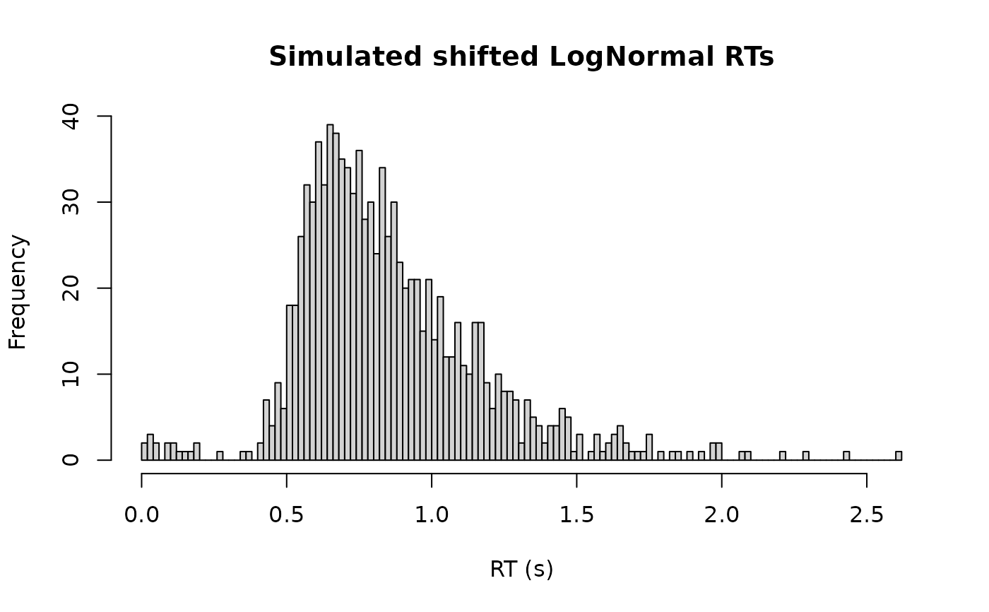
# Simulate 1000 RTs with 2% outliers
rts <- rcogmod_lognormal(1000, mu = -0.7, sigma = 0.5, ndt = 0.3, poutlier = 0.02)
hist(rts, breaks = 100, main = "Simulated shifted LogNormal RTs", xlab = "RT (s)")
 # Responses faster than ndt have positive density, unlike the unmixed model
dcogmod_lognormal(0.1, ndt = 0.3, poutlier = 0.02)
#> [1] 0.07041307
dcogmod_lognormal(0.1, ndt = 0.3, poutlier = 0)
#> [1] 0
# Density of the outlier component alone
curve(2 * dnorm(x, 0, 0.2), from = 0, to = 3, n = 1000)
# Responses faster than ndt have positive density, unlike the unmixed model
dcogmod_lognormal(0.1, ndt = 0.3, poutlier = 0.02)
#> [1] 0.07041307
dcogmod_lognormal(0.1, ndt = 0.3, poutlier = 0)
#> [1] 0
# Density of the outlier component alone
curve(2 * dnorm(x, 0, 0.2), from = 0, to = 3, n = 1000)