
Density, random generation, and brms custom family for the shifted
Inverse Gamma distribution. A Inverse Gamma-distributed decision time is shifted by a
non-decision time ndt, and a fixed proportion poutlier of responses is
generated by an outlier process instead of by the decision process.
Functions:
rcogmod_invgamma(): Simulates random draws.dcogmod_invgamma(): Computes the density (likelihood).pcogmod_invgamma(): Computes the cumulative distribution function (CDF) or survival.cogmod_invgamma(): Creates abrms::custom_family().cogmod_invgamma_stanvars(): Generates thestanvarsto pass tobrm().
Usage
rcogmod_invgamma(n, mu = 4, sigma = 1.5, ndt = 0.2, poutlier = 0)

dcogmod_invgamma(x, mu = 4, sigma = 1.5, ndt = 0.2, poutlier = 0, log = FALSE)

pcogmod_invgamma(
  q,
  mu = 4,
  sigma = 1.5,
  ndt = 0.2,
  poutlier = 0,
  lower.tail = TRUE,
  log.p = FALSE
)

cogmod_invgamma(
  link_mu = "softplus",
  link_sigma = "softplus",
  link_ndt = "log",
  link_poutlier = "logit",
  predict_outliers = FALSE
)

cogmod_invgamma_lpdf_expose()

cogmod_invgamma_stanvars()

log_lik_cogmod_invgamma(i, prep)

posterior_predict_cogmod_invgamma(i, prep, predict_outliers = NULL, ...)

posterior_epred_cogmod_invgamma(prep, predict_outliers = NULL)
Arguments
- n
Number of observations. If
length(n) > 1, the length is taken to be the number required.- mu
Shape of the inverse Gamma decision time. Must be positive.
- sigma
Scale of the inverse Gamma decision time. Must be positive.
- ndt
Non-decision time (shift parameter), in seconds. Must be non-negative. Represents time for processes such as stimulus encoding and response execution. Range: [0, Inf).
- poutlier
Proportion of responses generated by the outlier process rather than by the decision process. Range:
[0, 1]. Atpoutlier = 0the distribution reduces to the plain shifted LogNormal.- x
Vector of quantiles (observed reaction times).
- log
Logical; if TRUE, probabilities p are given as log(p).
- q
Vector of quantiles (reaction times, in seconds).
- lower.tail
Logical; if TRUE (default), probabilities are
P[X <= q], otherwiseP[X > q]- the survival, which is what a right-censored response contributes to the likelihood (see the Censoring section).- log.p
Logical; if TRUE, probabilities p are given as log(p).
- link_mu, link_sigma, link_ndt, link_poutlier
Link functions for the parameters.
- predict_outliers
Logical; whether
posterior_predict()andposterior_epred()should include the outlier component.FALSE(the default) fixespoutlierto zero for prediction, so predictions describe the decision process alone; the likelihood is always the full mixture either way. Seewith_outliers().- i, prep
For brms' functions to run: index of the observation and a
brmspreparation object.- ...
Additional arguments.
Value
rcogmod_invgamma() returns a numeric vector of n simulated
reaction times, in seconds. dcogmod_invgamma() returns the density at
each element of x - the log density if log = TRUE - recycled to the
length of the longest argument. cogmod_invgamma() returns a
brms::custom_family object, to put on a brms::bf() formula.
cogmod_invgamma_stanvars() returns a brms::stanvars object holding
the family's Stan functions block, to pass to brms::brm(), and
cogmod_invgamma_lpdf_expose() compiles that Stan code and returns it as
an R function, for checking the density outside of a model. The remaining
functions are brms post-processing methods, called by brms rather
than directly: log_lik_cogmod_invgamma() returns a numeric vector
holding one log-likelihood value per posterior draw for observation i,
and posterior_predict_cogmod_invgamma() a draws x 1 matrix of reaction
times simulated for observation i. posterior_epred_cogmod_invgamma()
returns a draws x observations matrix of expected reaction times, with
Inf wherever the mean does not exist.
Details
mu is the shape and sigma the scale of the inverse Gamma
decision time, whose mean is sigma / (mu - 1) and exists only for mu > 1.
ndt and poutlier mean exactly what they do in cogmod_lognormal(),
and with_outliers(), without_outliers(), p_outlier() and
cogmod_priors() all work here too. See ?rcogmod_lognormal for why ndt is
expressed directly in seconds rather than as a fraction of the fastest
observed response, what the half Normal outlier component is for, and why
the outlier component's scale is a constant rather than a dpar, and why
reaction times have to be in seconds.
posterior_epred() returns Inf where mu <= 1, because the inverse Gamma
has no mean there. The right tail is a power law, so this family is the one to
reach for when the slow tail is heavy; cogmod_loggamma() covers the same
territory continuously through negative shape.
Examples
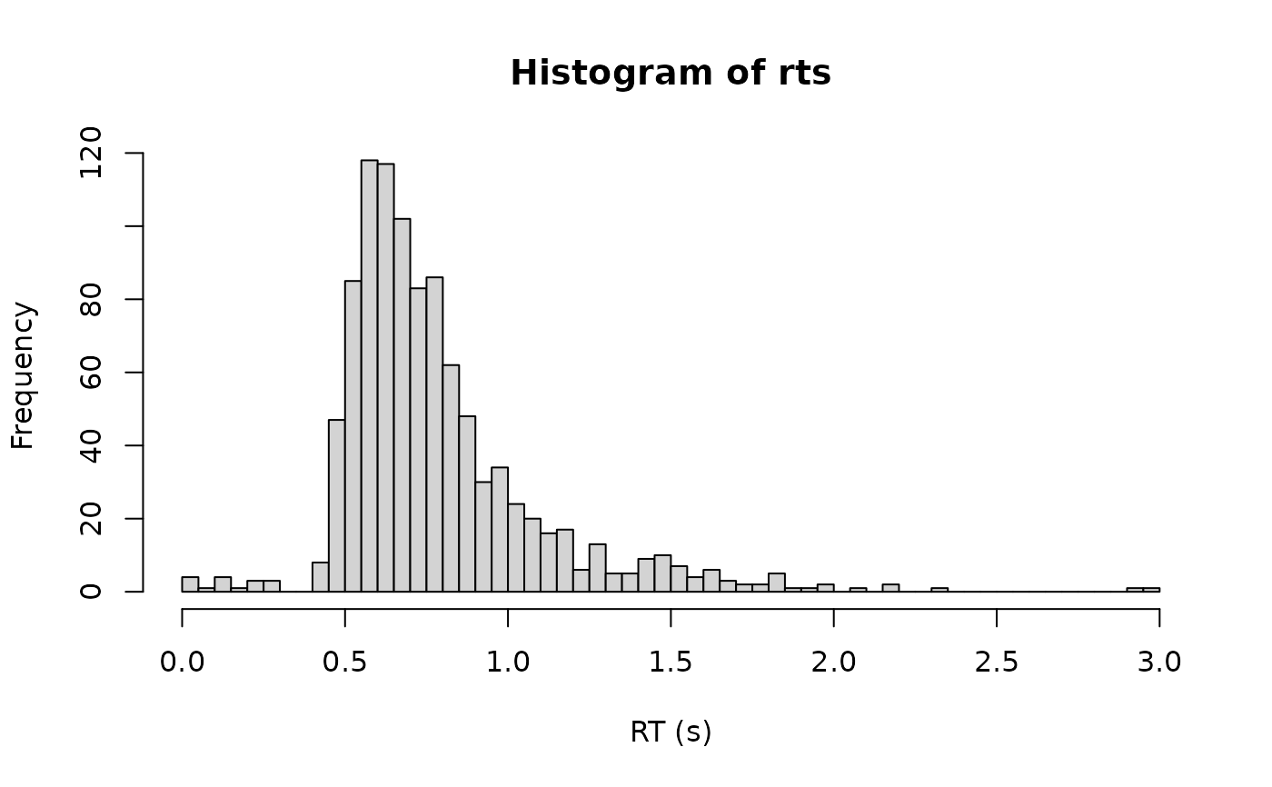
rts <- rcogmod_invgamma(1000, mu = 4, sigma = 1.5, ndt = 0.3, poutlier = 0.02)
hist(rts, breaks = 100, xlab = "RT (s)")
 # Responses faster than ndt keep positive density, unlike the unmixed model
dcogmod_invgamma(0.1, ndt = 0.3, poutlier = 0.02)
#> [1] 0.07041307
dcogmod_invgamma(0.1, ndt = 0.3, poutlier = 0)
#> [1] 0
# Responses faster than ndt keep positive density, unlike the unmixed model
dcogmod_invgamma(0.1, ndt = 0.3, poutlier = 0.02)
#> [1] 0.07041307
dcogmod_invgamma(0.1, ndt = 0.3, poutlier = 0)
#> [1] 0