Shifted Log-Gamma (Generalized Gamma) Model

Density, random generation, and brms custom family for the shifted Log-Gamma distribution. A Log-Gamma-distributed decision time is shifted by a non-decision time ndt, and a fixed proportion poutlier of responses is generated by an outlier process instead of by the decision process, exactly as in cogmod_lognormal().

Functions:

rcogmod_loggamma(): Simulates random draws from the shifted Log-Gamma model.
dcogmod_loggamma(): Computes the density (likelihood).
cogmod_loggamma(): Creates a brms::custom_family() for use in brms models.
cogmod_loggamma_stanvars(): Generates the stanvars to pass to brm().

Usage

rcogmod_loggamma(n, mu = -0.7, sigma = 0.5, shape = 0, ndt = 0.2, poutlier = 0)

dcogmod_loggamma(
  x,
  mu = -0.7,
  sigma = 0.5,
  shape = 0,
  ndt = 0.2,
  poutlier = 0,
  log = FALSE
)

cogmod_loggamma(
  link_mu = "identity",
  link_sigma = "softplus",
  link_shape = "identity",
  link_ndt = "log",
  link_poutlier = "logit",
  predict_outliers = FALSE
)

cogmod_loggamma_lpdf_expose()

cogmod_loggamma_stanvars()

log_lik_cogmod_loggamma(i, prep)

posterior_predict_cogmod_loggamma(i, prep, predict_outliers = NULL, ...)

posterior_epred_cogmod_loggamma(prep, predict_outliers = NULL)

Arguments

n: Number of observations. If length(n) > 1, the length is taken to be the number required.
mu: Location of the decision time on the log scale. Can take any real value. Range: (-Inf, Inf).
sigma: Scale of the decision time on the log scale. Must be positive. Range: (0, Inf).
shape: Shape (skewness) of the log-gamma on the log-RT scale. Unconstrained: shape = 0 is the LogNormal, shape = sigma the Gamma, shape = 1 the Weibull. See Details for the sigma * shape >= 1 boundary. Range: (-Inf, Inf).
ndt: Non-decision time (shift parameter), in seconds. Must be non-negative. Represents time for processes such as stimulus encoding and response execution. Range: [0, Inf).
poutlier: Proportion of responses generated by the outlier process rather than by the decision process. Range: [0, 1]. At poutlier = 0 the distribution reduces to the plain shifted LogNormal.
x: Vector of quantiles (observed reaction times).
log: Logical; if TRUE, probabilities p are given as log(p).
link_mu, link_sigma, link_shape, link_ndt, link_poutlier: Link functions for the parameters. shape is unconstrained and takes an identity link, so that the LogNormal (shape = 0) sits in the interior of its range rather than at a boundary.
predict_outliers: Logical; whether posterior_predict() and posterior_epred() should include the outlier component. FALSE (the default in cogmod_loggamma()) fixes poutlier to zero for prediction, so predictions describe the decision process alone; the likelihood is always the full mixture either way. On the prediction methods themselves the default is NULL, which defers to the flag carried on the model - see with_outliers() to change it after fitting.
i, prep: For brms' functions to run: index of the observation and a brms preparation object.
...: Additional arguments.

Value

rcogmod_loggamma() returns a numeric vector of n simulated reaction times, in seconds. dcogmod_loggamma() returns the density at each element of x - the log density if log = TRUE - recycled to the length of the longest argument. cogmod_loggamma() returns a brms::custom_family object, to put on a brms::bf() formula. cogmod_loggamma_stanvars() returns a brms::stanvars object holding the family's Stan functions block, to pass to brms::brm(), and cogmod_loggamma_lpdf_expose() compiles that Stan code and returns it as an R function, for checking the density outside of a model. The remaining functions are brms post-processing methods, called by brms rather than directly: log_lik_cogmod_loggamma() returns a numeric vector holding one log-likelihood value per posterior draw for observation i, and posterior_predict_cogmod_loggamma() a draws x 1 matrix of reaction times simulated for observation i. posterior_epred_cogmod_loggamma() returns a draws x observations matrix of expected reaction times.

What "Log-Gamma" means here

The log-gamma distribution is the distribution of log(G) for a Gamma variate G. Used as the distribution of the log decision time - in the same way the Normal is used in the shifted LogNormal - it gives a location-scale family on the log scale with one extra shape parameter:

log(RT - ndt) = mu + sigma * w,   w ~ standardized log-gamma with k = 1 / shape^2

Equivalently, RT - ndt follows a generalized gamma distribution (Stacy, 1962) in the parameterization of Prentice (1974), i.e. flexsurv::dgengamma(mu, sigma, Q = shape). The two names describe the same model: "log-gamma" names the distribution of log(RT - ndt), "generalized gamma" names the distribution of RT - ndt itself.

A two-parameter log-gamma is not a usable RT model, which is why there is a third parameter here. Exponentiating a plain two-parameter Gamma variate gives support on (1, Inf), so decision times would be forced above one second; adding a scale to fix that produces a second shift, perfectly confounded with ndt; and letting log(RT - ndt) be log-gamma with no location or scale just gives back the Gamma. Only the three-parameter location-scale-shape version is both non-degenerate and closed under a change of time unit (mu -> mu + log(c)), which everything else here relies on.

Relation to other "log-gamma" implementations

The name is used for two different distributions, and only one of them is this one.

scipy.stats.loggamma is the same distribution. It is log(G) for G ~ Gamma(c), with the usual loc and scale, so it is a three-parameter family exactly as this one is - c is the shape parameter, and it is not optional there either. Taking scipy's variate to be log(RT - ndt), the two line up exactly (verified to 3e-15):

c = 1 / shape^2      scale = sigma / shape      loc = mu + (sigma / shape) * log(shape^2)

Two deliberate differences. shape here is standardized so that the Normal limit sits at shape = 0, an interior point; in scipy's parameterization that limit is c -> Inf with loc and scale drifting off to compensate, which is not something a sampler can explore. And because scipy requires scale > 0, it covers only shape > 0; the shape < 0 half here - the inverse-Weibull side, with the power-law right tail - is the reflection, and would need -loggamma there.

actuar::dlgamma is a different distribution: exp(G) rather than log(G), hence its support of (1, Inf). That is the version with only two parameters, and the reason it needs only two is also the reason it is no use for reaction times - see the paragraph above on why exponentiating a Gamma does not give a usable RT model.

`shape`, and the families it nests

shape sets the skewness of the log-gamma on the log-RT scale; the Gamma it is the log of has its own shape k = 1 / shape^2. Throughout the docs below, "shape" unqualified means this parameter, never k.

It is unconstrained, with shape = 0 in the interior rather than at a boundary, which is what makes it usable as a free parameter:

`shape`	Distribution	right tail
`< -1`	heavier still than the inverse Weibull	power law
`= -1`	inverse Weibull (Frechet)	power law
`-1 to 0`	between the LogNormal and the inverse Weibull	power law
`= 0`	LogNormal - exactly `cogmod_lognormal()`	lognormal
`0 to 1`	between the LogNormal and the Weibull; Gamma (shape `1 / sigma^2`) at `shape = sigma`	lighter than lognormal
`= 1`	Weibull, shape `1 / sigma`	lighter than lognormal
`> 1`	lighter still than the Weibull	lightest

The right tail decays like exp(-c * t^(shape / sigma)) for shape > 0, so it thins monotonically as shape rises, and becomes a power law for shape < 0. shape therefore runs from heavy-tailed at the top of the table to light-tailed at the bottom, through the LogNormal in the middle. The Gamma sits inside 0 to 1 for any sigma < 1, which covers most RT data.

The model is therefore a strict generalisation of the shifted LogNormal, and fitting it is a way of testing whether the LogNormal shape is adequate: an interval for shape covering 0 says it is.

Where it misbehaves: `sigma * shape >= 1`

Just above the shift the decision density behaves like a Gamma whose own shape parameter is 1 / (sigma * shape). When sigma * shape >= 1 that Gamma shape falls below 1 and the density becomes unbounded at ndt, so the likelihood can be driven up without limit by pushing ndt toward the fastest response - the exact pathology the outlier component exists to remove, reintroduced through the shape parameter. The outlier component cannot repair it, because it adds density rather than capping it.

This is the same degeneracy the shifted Gamma and shifted Weibull have when their own shape falls below 1; it is inherited here, not introduced. In practice the prior on shape is what keeps you out of it: cogmod_priors() uses normal(0, 0.5) on the intercept, which for a typical sigma around 0.5 leaves the boundary at shape = 2, four prior SDs away. A posterior for shape pushing up against 1 / sigma is the model asking for a spike at the shift, not for a decision-time distribution.

Negative shape has the mirror-image caveat: the right tail is a power law, and the mean of the decision component is finite only when sigma * abs(shape) < 1. posterior_epred() returns Inf where it is not.

Fit with `init = 0`

The prior keeps the posterior clear of that boundary, but it does not control where a chain starts. brms initialises on the unconstrained scale from U(-2, 2), which for the default links puts shape in (-2, 2) and sigma in (0.13, 2.13) - and about 15% of chains start with sigma * shape >= 1. A chain starting inside the unbounded region falls into the spike at ndt and does not come back out: it does not error, it simply runs for as long as you let it while the others finish.

init = 0 removes the problem by construction, starting every chain at shape = 0 - the LogNormal - with sigma * shape = 0:

f <- brms::bf(RT ~ 1, sigma ~ 1, shape ~ 1, ndt ~ 1, poutlier ~ 1,
              family = cogmod_loggamma())
brms::brm(f, data = df,
          prior = cogmod_priors(f, df),
          stanvars = cogmod_stanvars(f),
          init = 0)

This is not a tuning suggestion to try if sampling looks bad; it is how the model should be fitted. The one visible symptom of getting it wrong is a chain that never finishes.

`ndt` and `poutlier`

Identical in meaning, parameterization and defaults to cogmod_lognormal() - see its Details for the full account of why ndt is expressed directly in seconds, what the half Normal outlier component is for, why its scale is a constant rather than a dpar, and why predictions exclude the outlier component by default. with_outliers(), without_outliers(), p_outlier() and cogmod_priors() all work on this family too.

References

Stacy, E. W. (1962). A generalization of the gamma distribution. The Annals of Mathematical Statistics, 33(3), 1187-1192. doi:10.1214/aoms/1177704481

Prentice, R. L. (1974). A log gamma model and its maximum likelihood estimation. Biometrika, 61(3), 539-544. doi:10.1093/biomet/61.3.539

Examples

# shape = 0 is exactly the shifted LogNormal
dcogmod_loggamma(0.9, mu = -0.7, sigma = 0.5, shape = 0, ndt = 0.3)
#> [1] 1.237954
dcogmod_lognormal(0.9, mu = -0.7, sigma = 0.5, ndt = 0.3)
#> [1] 1.237954

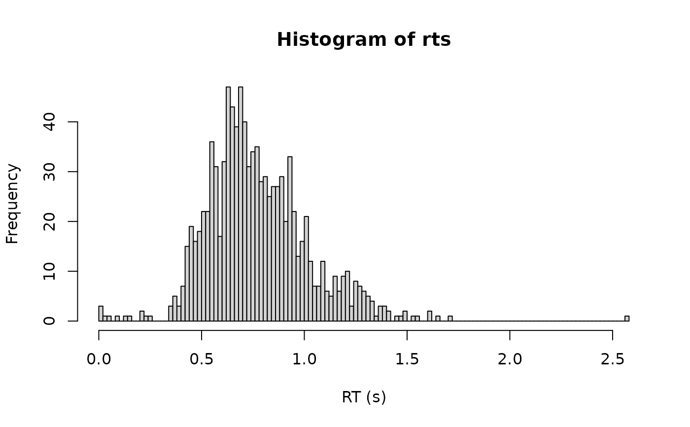
# Simulate 1000 RTs with 2% outliers and a slightly Gamma-like shape
rts <- rcogmod_loggamma(1000,
  mu = -0.7, sigma = 0.5, shape = 0.5, ndt = 0.3,
  poutlier = 0.02
)
hist(rts, breaks = 100, xlab = "RT (s)")


# Responses faster than ndt keep positive density, as in cogmod_lognormal()
dcogmod_loggamma(0.1, ndt = 0.3, poutlier = 0.02)
#> [1] 0.07041307
dcogmod_loggamma(0.1, ndt = 0.3, poutlier = 0)
#> [1] 0

# shape = sigma is the shifted Gamma, with shape 1 / sigma^2
dcogmod_loggamma(0.9, mu = -0.7, sigma = 0.5, shape = 0.5, ndt = 0.3)
#> [1] 1.206755
stats::dgamma(0.6, shape = 4, scale = exp(-0.7) * 0.25)
#> [1] 1.206755