Shifted Weibull Model — rcogmod

Density, random generation, and brms custom family for the shifted Weibull distribution. A Weibull-distributed decision time is shifted by a non-decision time ndt, and a fixed proportion poutlier of responses is generated by an outlier process instead of by the decision process.

Functions:

rcogmod_weibull(): Simulates random draws.
dcogmod_weibull(): Computes the density (likelihood).
pcogmod_weibull(): Computes the cumulative distribution function (CDF) or survival.
cogmod_weibull(): Creates a brms::custom_family().
cogmod_weibull_stanvars(): Generates the stanvars to pass to brm().

Usage

rcogmod_weibull(n, mu = 2, sigma = 0.5, ndt = 0.2, poutlier = 0)

dcogmod_weibull(x, mu = 2, sigma = 0.5, ndt = 0.2, poutlier = 0, log = FALSE)

pcogmod_weibull(
  q,
  mu = 2,
  sigma = 0.5,
  ndt = 0.2,
  poutlier = 0,
  lower.tail = TRUE,
  log.p = FALSE
)

cogmod_weibull(
  link_mu = "softplus",
  link_sigma = "softplus",
  link_ndt = "log",
  link_poutlier = "logit",
  predict_outliers = FALSE
)

cogmod_weibull_lpdf_expose()

cogmod_weibull_stanvars()

log_lik_cogmod_weibull(i, prep)

posterior_predict_cogmod_weibull(i, prep, predict_outliers = NULL, ...)

posterior_epred_cogmod_weibull(prep, predict_outliers = NULL)

Arguments

n: Number of observations. If length(n) > 1, the length is taken to be the number required.
mu: Shape of the Weibull decision time. Must be positive.
sigma: Scale of the Weibull decision time. Must be positive.
ndt: Non-decision time (shift parameter), in seconds. Must be non-negative. Represents time for processes such as stimulus encoding and response execution. Range: [0, Inf).
poutlier: Proportion of responses generated by the outlier process rather than by the decision process. Range: [0, 1]. At poutlier = 0 the distribution reduces to the plain shifted LogNormal.
x: Vector of quantiles (observed reaction times).
log: Logical; if TRUE, probabilities p are given as log(p).
q: Vector of quantiles (reaction times, in seconds).
lower.tail: Logical; if TRUE (default), probabilities are P[X <= q], otherwise P[X > q] - the survival, which is what a right-censored response contributes to the likelihood (see the Censoring section).
log.p: Logical; if TRUE, probabilities p are given as log(p).
link_mu, link_sigma, link_ndt, link_poutlier: Link functions for the parameters.
predict_outliers: Logical; whether posterior_predict() and posterior_epred() should include the outlier component. FALSE (the default) fixes poutlier to zero for prediction, so predictions describe the decision process alone; the likelihood is always the full mixture either way. See with_outliers().
i, prep: For brms' functions to run: index of the observation and a brms preparation object.
...: Additional arguments.

Value

rcogmod_weibull() returns a numeric vector of n simulated reaction times, in seconds. dcogmod_weibull() returns the density at each element of x - the log density if log = TRUE - recycled to the length of the longest argument. cogmod_weibull() returns a brms::custom_family object, to put on a brms::bf() formula. cogmod_weibull_stanvars() returns a brms::stanvars object holding the family's Stan functions block, to pass to brms::brm(), and cogmod_weibull_lpdf_expose() compiles that Stan code and returns it as an R function, for checking the density outside of a model. The remaining functions are brms post-processing methods, called by brms rather than directly: log_lik_cogmod_weibull() returns a numeric vector holding one log-likelihood value per posterior draw for observation i, and posterior_predict_cogmod_weibull() a draws x 1 matrix of reaction times simulated for observation i. posterior_epred_cogmod_weibull() returns a draws x observations matrix of expected reaction times.

Details

mu is the shape and sigma the scale of the Weibull decision time, whose mean is sigma * gamma(1 + 1 / mu).

ndt and poutlier mean exactly what they do in cogmod_lognormal(), and with_outliers(), without_outliers(), p_outlier() and cogmod_priors() all work here too. See ?rcogmod_lognormal for why ndt is expressed directly in seconds rather than as a fraction of the fastest observed response, what the half Normal outlier component is for, and why the outlier component's scale is a constant rather than a dpar, and why reaction times have to be in seconds.

The shape governs how well this samples

Near the shift the Weibull density behaves like (y - ndt)^(mu - 1), and that exponent decides how the mixture behaves as ndt passes an observation. Three regimes, in order of severity:

mu < 1: the density is unbounded at ndt, so the likelihood is unbounded as ndt approaches the fastest response. The outlier component adds density rather than capping it, so it cannot repair that.
mu < 2: the density is bounded, but the derivative of the log-likelihood with respect to ndt behaves like (y - ndt)^(mu - 2) and so is unbounded at every observation. The posterior is proper - poutlier keeps it so - but the gradient spikes wherever ndt sits close to a response, which is exactly where the data put it.
mu > 2: bounded gradient. mu > 3 additionally bounds the curvature.

The middle regime is the one to watch, because nothing warns about it. On the 4285-trial lexical-decision data in vignette("rt_models") the shape comes out at 1.4, ndt lands at 0.40 s inside the dense left edge of the data, and the sampler's step size collapses to 0.005 against 0.19 for cogmod_lognormal() on the same data: mean treedepth 8.1 against 3.9, which is 19x the gradient evaluations and 19x the wall time, with Rhat 1.18 on ndt. The density itself is cheap; all of the cost is geometry.

What does not help

All of the obvious remedies were tried on that fit and measured. None of them works, and two make it worse, so they are recorded here rather than left for the next person to rediscover.

A prior on the shape. normal(2.4, 0.4) on the softplus scale puts 95% of its mass above mu = 1.9. It moved the posterior shape by 0.01, because the likelihood prefers the low-shape corner by around 100 log units and the prior contributes 5.

A narrow prior on ndt. This looks like the obvious fix - keep the shift below the data and the singular region is never visited - and it fails for an instructive reason. normal(-1.25, 0.05), centred at 0.287 s with 95% of its mass below the fastest bulk response, left the posterior at 0.396 s: 6.5 prior SDs away, essentially where it was without any prior at all. The ndt likelihood has a posterior SD of 0.003, so it is some fifteen times sharper than that prior; nothing weaker than fixing ndt outright competes with it. What the attempt did achieve was 4% divergent transitions against 0.5%, 16% of iterations at maximum treedepth against 7%, Rhat 1.43 against 1.18, and a slightly worse loo.

Fixing ndt at the fastest observed response. This does remove the problem, by removing the parameter - but it reinstates exactly the min-RT bound this parameterization exists to get rid of, and it is unsound wherever the outlier component is doing its job. On the data above the fastest response is 71 ms, which is not a decision; the mixture is there precisely so that an order statistic of the sample is not treated as a bound. See cogmod_lognormal().

Note also what is not wrong: ndt and the shape are jointly identified, and sharply so - the posterior SD on ndt is 3 ms. This is not a case of two parameters trading off with nothing to separate them, so pinning one of them is not the missing ingredient. The sharpness simply sits on a ridge that is not smooth.

What to do instead

Treat a fitted shape below 2 as the diagnostic it is, and use cogmod_loggamma(), which nests this family at shape = 1 and lets the data choose the shape rather than having the family fix it. On the data above it samples in a third of the time with no divergences.

The slow sampling and the poor fit are the same fact, not two problems. Across the ten families fitted in vignette("rt_models") the Weibull comes last by loo, 196 elpd (SE 21) behind cogmod_loggamma() and 95 behind the next worst. What the sampler struggles with is the model contorting itself - pushing the shift up into the data, pulling the shape toward 1 - to represent a left edge it cannot otherwise reach. That does not make the Weibull useless for reaction times in general; where the shape comes out above 2 the family is perfectly well behaved, as cogmod_gamma() is on these same data at a shape of 2.2. It does mean a shape below 2 should be read as the model telling you to use a different one.

Under the older ndt = tau * min(RT) parameterization the problem was hidden rather than absent: the logit Jacobian vanished as tau approached 1, which damped exactly this gradient.

Starting values

Do not fit this with init = 0: it puts ndt at exp(0) = 1 second and the shape at softplus(0) = 0.69, inside the mu < 1 regime above, and no single scalar avoids both. Use cogmod_inits(), which sets them separately:

brms::brm(f, data = df, prior = cogmod_priors(f, df),
          stanvars = cogmod_stanvars(f), init = cogmod_inits(f, df))

See cogmod_inits() for why, and ?rcogmod_gamma for what it costs when ignored.

Examples

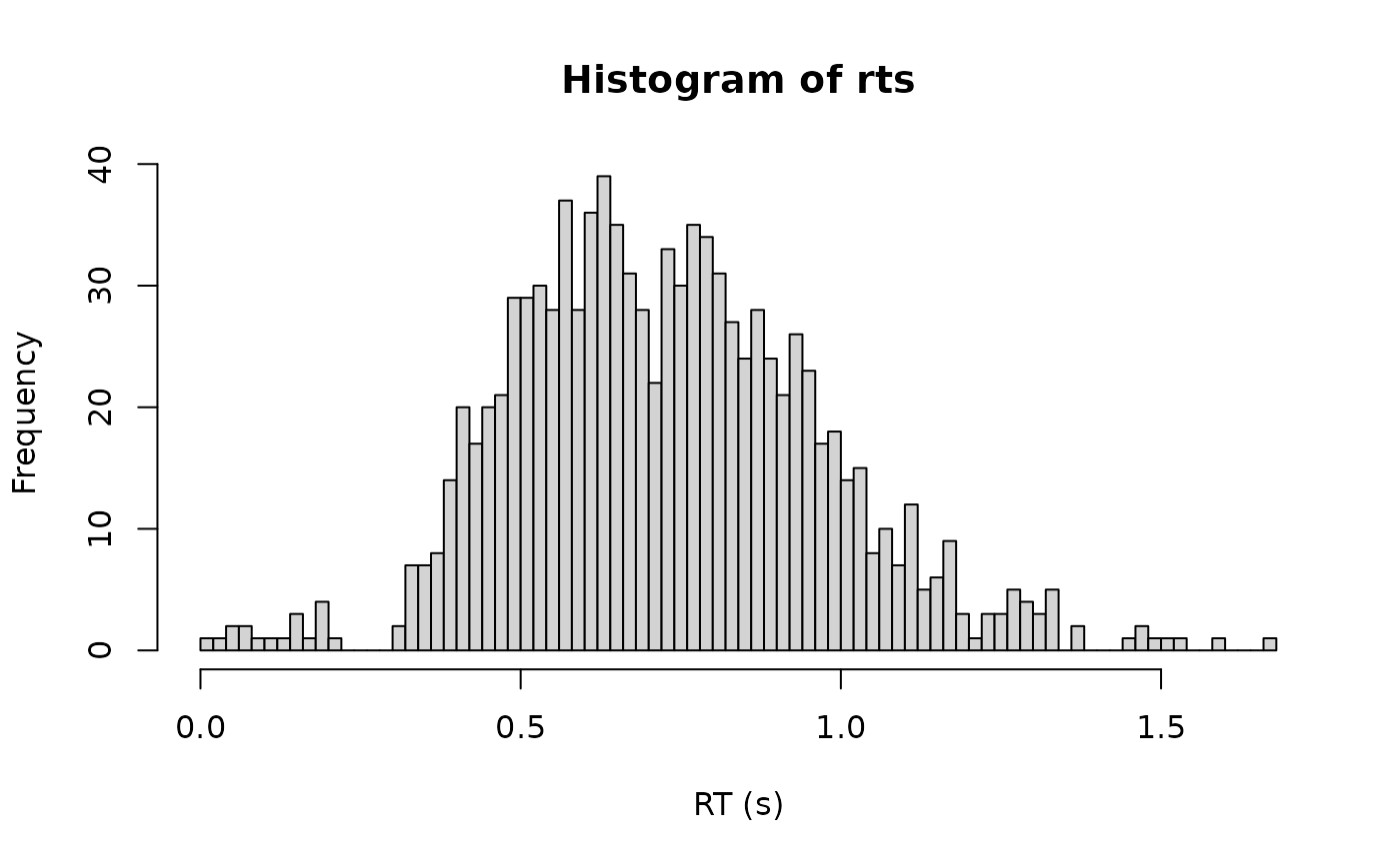
rts <- rcogmod_weibull(1000, mu = 2, sigma = 0.5, ndt = 0.3, poutlier = 0.02)
hist(rts, breaks = 100, xlab = "RT (s)")


# Responses faster than ndt keep positive density, unlike the unmixed model
dcogmod_weibull(0.1, ndt = 0.3, poutlier = 0.02)
#> [1] 0.07041307
dcogmod_weibull(0.1, ndt = 0.3, poutlier = 0)
#> [1] 0