Shifted Birnbaum-Saunders (Fatigue Life) Model

Density, random generation, and brms custom family for the shifted Birnbaum-Saunders distribution, also known as the fatigue life distribution: a first-passage-time model in which evidence arrives in discrete cycles and only ever towards the boundary. The decision time is shifted by a non-decision time ndt, and a fixed proportion poutlier of responses is generated by an outlier process instead of by the decision process.

Functions:

rcogmod_bisa(): Simulates random draws.
dcogmod_bisa(): Computes the density (likelihood).
pcogmod_bisa(): Computes the cumulative distribution function (CDF) or survival.
cogmod_bisa(): Creates a brms::custom_family().
cogmod_bisa_stanvars(): Generates the stanvars to pass to brm().

Usage

rcogmod_bisa(n, mu = 3, boundary = 0.5, ndt = 0.2, poutlier = 0)

dcogmod_bisa(x, mu = 3, boundary = 0.5, ndt = 0.2, poutlier = 0, log = FALSE)

pcogmod_bisa(
  q,
  mu = 3,
  boundary = 0.5,
  ndt = 0.2,
  poutlier = 0,
  lower.tail = TRUE,
  log.p = FALSE
)

cogmod_bisa(
  link_mu = "softplus",
  link_boundary = "softplus",
  link_ndt = "log",
  link_poutlier = "logit",
  predict_outliers = FALSE
)

cogmod_bisa_lpdf_expose()

cogmod_bisa_stanvars()

log_lik_cogmod_bisa(i, prep)

posterior_predict_cogmod_bisa(i, prep, predict_outliers = NULL, ...)

posterior_epred_cogmod_bisa(prep, predict_outliers = NULL)

Arguments

n: Number of observations. If length(n) > 1, the length is taken to be the number required.
mu: Drift rate: the average size of the per-cycle evidence increment, whose SD is fixed at 1. Must be positive.
boundary: Decision threshold: the evidence needed to respond. Must be positive.
ndt: Non-decision time (shift parameter), in seconds. Must be non-negative. Represents time for processes such as stimulus encoding and response execution. Range: [0, Inf).
poutlier: Proportion of responses generated by the outlier process rather than by the decision process. Range: [0, 1]. At poutlier = 0 the distribution reduces to the plain shifted LogNormal.
x: Vector of quantiles (observed reaction times).
log: Logical; if TRUE, probabilities p are given as log(p).
q: Vector of quantiles (reaction times, in seconds).
lower.tail: Logical; if TRUE (default), probabilities are P[X <= q], otherwise P[X > q] - the survival, which is what a right-censored response contributes to the likelihood (see the Censoring section).
log.p: Logical; if TRUE, probabilities p are given as log(p).
link_mu, link_boundary, link_ndt, link_poutlier: Link functions for the parameters.
predict_outliers: Logical; whether posterior_predict() and posterior_epred() should include the outlier component. FALSE (the default) fixes poutlier to zero for prediction, so predictions describe the decision process alone; the likelihood is always the full mixture either way. See with_outliers().
i, prep: For brms' functions to run: index of the observation and a brms preparation object.
...: Additional arguments.

Value

rcogmod_bisa() returns a numeric vector of n simulated reaction times, in seconds. dcogmod_bisa() returns the density at each element of x - the log density if log = TRUE - recycled to the length of the longest argument. cogmod_bisa() returns a brms::custom_family object, to put on a brms::bf() formula. cogmod_bisa_stanvars() returns a brms::stanvars object holding the family's Stan functions block, to pass to brms::brm(), and cogmod_bisa_lpdf_expose() compiles that Stan code and returns it as an R function, for checking the density outside of a model. The remaining functions are brms post-processing methods, called by brms rather than directly: log_lik_cogmod_bisa() returns a numeric vector holding one log-likelihood value per posterior draw for observation i, and posterior_predict_cogmod_bisa() a draws x 1 matrix of reaction times simulated for observation i. posterior_epred_cogmod_bisa() returns a draws x observations matrix of expected reaction times.

Details

The Birnbaum-Saunders distribution is the near neighbour of the Wald (cogmod_invgaussian()), and this family is deliberately parameterized so that the two can be compared directly: mu is a drift rate and boundary a decision threshold in both, meaning the same thing, so the only thing that differs between them is how the evidence arrives.

ndt and poutlier mean exactly what they do in cogmod_lognormal(), and with_outliers(), without_outliers(), p_outlier() and cogmod_priors() all work here too. See ?rcogmod_lognormal for why ndt is expressed directly in seconds, what the outlier component is for, and why its scale is a constant rather than a dpar.

Where the distribution comes from

A Wald time is the first crossing of a diffusion: evidence moves continuously and can move either way at any instant. Here it instead accumulates in discrete cycles, and every cycle pushes towards the boundary - what is random is the size of each increment, never its sign. If the increments have average size mu and SD 1, then after n cycles the accumulated evidence is Normal(n * mu, n) by the central limit theorem, so

P(T <= n) = P(evidence >= boundary) = Phi((mu * n - boundary) / sqrt(n))

and treating the cycle count n as continuous turns that into a first-crossing time. It is one-directional accumulation in discrete chunks, with a Gaussian approximation standing in for the exact hitting-time calculation - which is exactly the fatigue-crack process Birnbaum and Saunders (1969) derived it for.

Fixing the per-cycle SD at 1 is not an arbitrary choice: it is the same convention that fixes the Wald's diffusion coefficient, and it is what keeps mu and boundary on a common scale across the two families. It also means there is no third parameter and there cannot be one - the shape is pinned by mu * boundary, just as the Wald's shape is pinned at boundary^2.

The tidy consequence is that

(mu * t - boundary) / sqrt(t)

is exactly standard normal. In the distribution's usual (a, b) parameters that transform is written (1 / a) * (sqrt(t / b) - sqrt(b / t)), with scale b = boundary / mu and shape a = 1 / sqrt(mu * boundary). The map between the two parameterizations is a bijection - boundary = sqrt(b) / a and mu = 1 / (a * sqrt(b)) - so nothing is given up by stating it mechanistically. Every quantity of the family is elementary as a result: the CDF is a normal CDF, the quantile function a closed form, and rcogmod_bisa() is one normal draw per observation with no rejection step.

Relation to the Wald

In these parameters the density is the Wald's own, tilted:

f_BS(t) = f_Wald(t; mu, boundary) * (mu * t + boundary) / (2 * boundary)

One sign is all that separates them - the exponent carries (mu * t - boundary), the prefactor (mu * t + boundary). The tilt factor is what makes the Birnbaum-Saunders an equal mixture of an inverse Gaussian and a reciprocal inverse Gaussian: half the mass is the Wald with the same mu and boundary, half is that Wald's length-biased version, which weights long crossings in proportion to their length.

So at the same (mu, boundary) this family is both slower and more spread out than the Wald. At mu = 3, boundary = 0.5 its mean is 0.222 s against the Wald's 0.167, and its SD 0.184 against 0.136. In general

E[T]   = boundary / mu   + 1 / (2 * mu^2)    # the Wald's mean, plus a term
Var[T] = boundary / mu^3 + 5 / (4 * mu^4)    # the Wald's variance, plus one

both always finite, so posterior_epred() always has a number to return - unlike cogmod_invgaussian() once its drift varies. The median is exactly boundary / mu, which is the Wald's mean: do not read the two families' parameters as describing the same central tendency.

The right tail decays like exp(-mu^2 * t / 2), the same exponential order as the Wald's and much lighter than a LogNormal's, and the density vanishes at the shift with all its derivatives. ndt is therefore as well behaved here as it is for the Wald, with no unbounded-likelihood boundary of the kind cogmod_gamma() and cogmod_weibull() have at shape < 1.

There is no sigmadrift. Across-trial drift variability is what cogmod_invgaussian() is for; here the extra dispersion comes from the mixture structure instead, at no cost in parameters.

References

Birnbaum, Z. W., & Saunders, S. C. (1969). A new family of life distributions. Journal of Applied Probability, 6(2), 319-327. doi:10.2307/3212003
Desmond, A. F. (1986). On the relationship between two fatigue-life models. IEEE Transactions on Reliability, R-35(2), 167-169. doi:10.1109/TR.1986.4335400

Examples

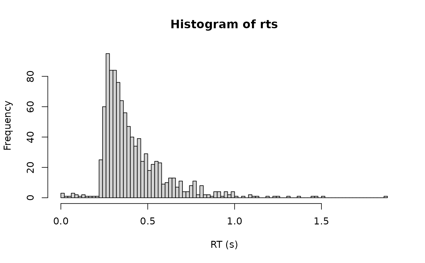
rts <- rcogmod_bisa(1000, mu = 3, boundary = 0.5, ndt = 0.2, poutlier = 0.02)
hist(rts, breaks = 100, xlab = "RT (s)")


# The mean is the Wald's, boundary / mu, plus 1 / (2 * mu^2).
mean(rcogmod_bisa(1e5, mu = 3, boundary = 0.5, ndt = 0.2))
#> [1] 0.4224397
0.2 + 0.5 / 3 + 1 / (2 * 3^2)
#> [1] 0.4222222

# The median is exactly ndt + boundary / mu.
median(rcogmod_bisa(1e5, mu = 3, boundary = 0.5, ndt = 0.2))
#> [1] 0.3669211