
Density, random generation, and brms custom family for the shifted ex-Wald
distribution of Schwarz (2001): a Wald (diffusive) decision stage convolved
with an exponential residual stage. The decision time is shifted by a
non-decision time ndt, and a fixed proportion poutlier of responses is
generated by an outlier process instead of by the decision process.
Functions:
rcogmod_exwald(): Simulates random draws.dcogmod_exwald(): Computes the density (likelihood).cogmod_exwald(): Creates abrms::custom_family().cogmod_exwald_stanvars(): Generates thestanvarsto pass tobrm().
Usage
rcogmod_exwald(n, mu = 3, boundary = 0.5, tau = 0.15, ndt = 0.2, poutlier = 0)

dcogmod_exwald(
  x,
  mu = 3,
  boundary = 0.5,
  tau = 0.15,
  ndt = 0.2,
  poutlier = 0,
  log = FALSE
)

cogmod_exwald(
  link_mu = "softplus",
  link_boundary = "softplus",
  link_tau = "softplus",
  link_ndt = "log",
  link_poutlier = "logit",
  predict_outliers = FALSE
)

cogmod_exwald_lpdf_expose()

cogmod_exwald_stanvars()

log_lik_cogmod_exwald(i, prep)

posterior_predict_cogmod_exwald(i, prep, predict_outliers = NULL, ...)

posterior_epred_cogmod_exwald(prep, predict_outliers = NULL)
Arguments
- n
Number of observations. If
length(n) > 1, the length is taken to be the number required.- mu
Drift rate: the average speed of evidence accumulation. Must be positive.
- boundary
Decision threshold: the evidence needed to respond. Must be positive.
- tau
Mean of the exponential residual stage, in seconds. Must be positive.
- ndt
Non-decision time (shift parameter), in seconds. Must be non-negative. Represents time for processes such as stimulus encoding and response execution. Range: [0, Inf).
- poutlier
Proportion of responses generated by the outlier process rather than by the decision process. Range:
[0, 1]. Atpoutlier = 0the distribution reduces to the plain shifted LogNormal.- x
Vector of quantiles (observed reaction times).
- log
Logical; if TRUE, probabilities p are given as log(p).
- link_mu, link_boundary, link_tau, link_ndt, link_poutlier
Link functions for the parameters.
- predict_outliers
Logical; whether
posterior_predict()andposterior_epred()should include the outlier component.FALSE(the default) fixespoutlierto zero for prediction, so predictions describe the decision process alone; the likelihood is always the full mixture either way. Seewith_outliers().- i, prep
For brms' functions to run: index of the observation and a
brmspreparation object.- ...
Additional arguments.
Value
rcogmod_exwald() returns a numeric vector of n simulated
reaction times, in seconds. dcogmod_exwald() returns the density at
each element of x - the log density if log = TRUE - recycled to the
length of the longest argument. cogmod_exwald() returns a
brms::custom_family object, to put on a brms::bf() formula.
cogmod_exwald_stanvars() returns a brms::stanvars object holding the
family's Stan functions block, to pass to brms::brm(), and
cogmod_exwald_lpdf_expose() compiles that Stan code and returns it as
an R function, for checking the density outside of a model. The remaining
functions are brms post-processing methods, called by brms rather
than directly: log_lik_cogmod_exwald() returns a numeric vector holding
one log-likelihood value per posterior draw for observation i, and
posterior_predict_cogmod_exwald() a draws x 1 matrix of reaction times
simulated for observation i. posterior_epred_cogmod_exwald() returns
a draws x observations matrix of expected reaction times.
Details
The decision time is Wald(mu, boundary) + Exponential(1 / tau): evidence
accumulates at rate mu until it reaches boundary, and an exponentially
distributed residual stage of mean tau follows. It is the mechanistic
counterpart of cogmod_exgaussian(), whose first stage is a descriptive
Gaussian rather than a decision process, and tau means the same thing in
both.
ndt and poutlier mean exactly what they do in cogmod_lognormal(),
and with_outliers(), without_outliers(), p_outlier() and
cogmod_priors() all work here too. See ?rcogmod_lognormal for why ndt is
expressed directly in seconds, what the outlier component is for, and why its
scale is a constant rather than a dpar.
The mean exists and is ndt + boundary / mu + tau, so posterior_epred()
returns a number - unlike cogmod_invgaussian() once its drift varies.
ndt and tau
Both delay the response, and they are separated only by shape: ndt is a
hard floor, tau a variable stage with an exponential spread. That makes
them a ridge rather than a flat direction - the leading edge of the
distribution identifies ndt - but a ridge all the same. The normal(-1.2, 0.2) that cogmod_priors() puts on ndt is what holds it; widen it and
expect the two to trade off. Schwarz's own model has no ndt at all, the
exponential stage being the whole of the residual time, and fixing ndt = 0
in bf() recovers exactly that.
There is deliberately no sigmadrift. It and tau both fatten the right
tail and are very hard to tell apart; cogmod_invgaussian() is where the
drift-variability route lives.
How the density is computed
Worth knowing, because the two branches are not equally common. Writing
g = 1 / tau, the convolution has an elementary closed form,
g * exp(-g * t + boundary * (mu - k)) * F_Wald(t; k, boundary) with
k = sqrt(mu^2 - 2 * g), whenever mu^2 > 2 / tau. At a drift of 3 and a
threshold of 0.5 that asks for tau > 0.22 s, where a residual stage is more
often nearer 0.1 s, so the other branch is reached routinely.
There k is imaginary, and the same expression continues analytically into
g * exp(-(boundary - mu * t)^2 / (2 * t)) * Re[w(z)], where w is the
Faddeeva function and z = (kappa * sqrt(t) + i * boundary / sqrt(t)) / sqrt(2) with kappa = sqrt(2 / tau - mu^2). The exponent is the Wald's own,
so nothing overflows, and w is evaluated by Weideman's 24-term rational
approximation. Both branches are exact, and they meet exactly at
mu^2 = 2 / tau - at kappa = 0 the second reduces to the first - so the
relative step measured either side of the seam is 5e-8, which is rounding.
Quadrature on the original convolution integral was tried first and does not
work: the log-integrand is bimodal, with one peak at the Wald bulk near zero
and another at u = t where exp(u / tau) is climbing, and their widths vary
independently over orders of magnitude. Fixed-panel rules reach only 1e-1
relative error somewhere in the region an RT fit actually visits, and leave a
step of 0.74 at the seam.
References
Schwarz, W. (2001). The ex-Wald distribution as a descriptive model of response times. Behavior Research Methods, Instruments, & Computers, 33(4), 457-469. doi:10.3758/bf03195403
Examples
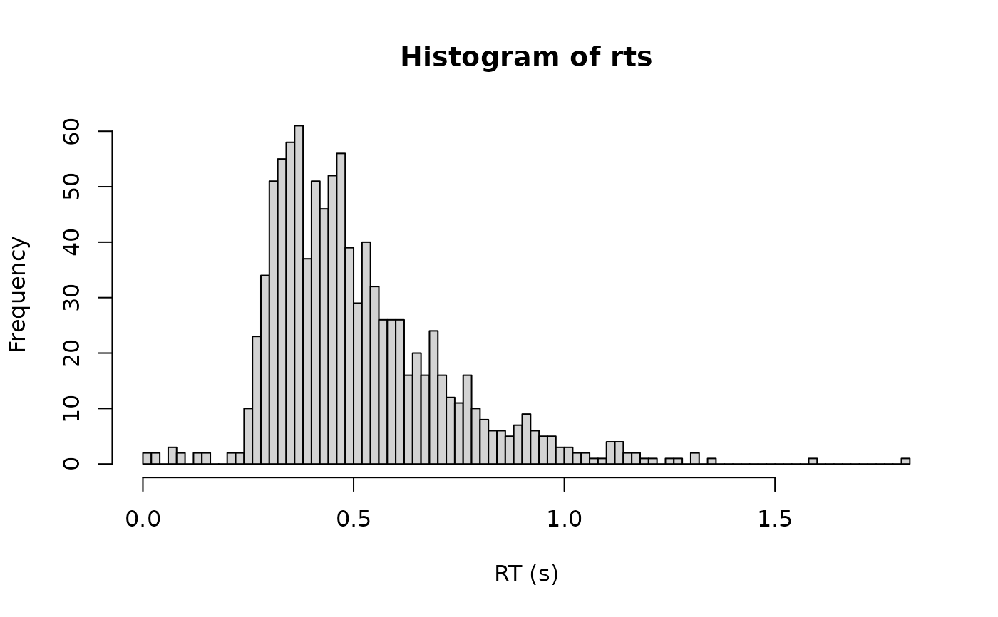
rts <- rcogmod_exwald(1000, mu = 3, boundary = 0.5, tau = 0.15,
ndt = 0.2, poutlier = 0.02)
hist(rts, breaks = 100, xlab = "RT (s)")
 # The mean is boundary / mu + tau, on top of ndt.
mean(rcogmod_exwald(1e5, mu = 3, boundary = 0.5, tau = 0.15, ndt = 0.2))
#> [1] 0.5165326
0.2 + 0.5 / 3 + 0.15
#> [1] 0.5166667
# The mean is boundary / mu + tau, on top of ndt.
mean(rcogmod_exwald(1e5, mu = 3, boundary = 0.5, tau = 0.15, ndt = 0.2))
#> [1] 0.5165326
0.2 + 0.5 / 3 + 0.15
#> [1] 0.5166667